El siguiente programa nos permite visualizar los modos guiados. Para eso es necesario dar exactamente el vector de onda y frecuencia, los cuales se pueden obtener del post anterior.
Separamos en un programa par y otro programa impar.
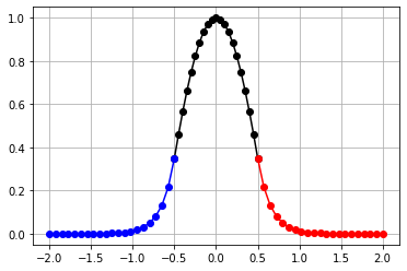
Modos par
qlx=13033816.300340246
khx=4849447.026609609

xi      = -d/2
xf      =  d/2
Nx      = 20
dx      = (xf-xi)/Nx

xVc      = np.zeros(Nx+1)
aux5    = np.zeros(Nx+1)
aux6    = np.zeros(Nx+1)

for ix in range(0,Nx+1):
  x        = xi+ix*dx
  xVc[ix]   = x/d
  aux5[ix] = math.cos(khx*x)

A=math.cos(khx*0.5*d)/math.exp(-qlx*0.5*d)
D=math.cos(khx*0.5*d)/math.exp(-qlx*0.5*d)
xi      = -2*d
xf      = -d/2
Nx      = 20
dx      = (xf-xi)/Nx

xVl     = np.zeros(Nx+1)
aux7    = np.zeros(Nx+1)
aux8    = np.zeros(Nx+1)

for ix in range(0,Nx+1):
  x        = xi+ix*dx
  xVl[ix]  = x/d
  aux7[ix] = A*math.exp(qlx*x)

xi      = d/2
xf      = 2*d
Nx      = 20
dx      = (xf-xi)/Nx

xVr     = np.zeros(Nx+1)
aux9    = np.zeros(Nx+1)
aux10   = np.zeros(Nx+1)

for ix in range(0,Nx+1):
  x        = xi+ix*dx
  xVr[ix]  = x/d
  aux9[ix] = D*math.exp(-qlx*x)

plt.plot(xVc,aux5,'ko-')
plt.plot(xVl,aux7,'bo-')
plt.plot(xVr,aux9,'ro-')
plt.grid()
plt.show()
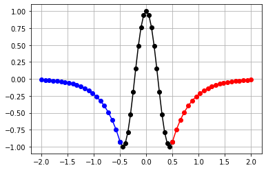
Podemos ver el segundo modo par si ponemos
qlx=5627974.468371605
khx=14131002.155258968
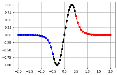
Modo impar
qlx=11596990.03063907
khx=9842212.18821431

xi      = -d/2
xf      =  d/2
Nx      = 20
dx      = (xf-xi)/Nx

xVc      = np.zeros(Nx+1)
aux5    = np.zeros(Nx+1)
aux6    = np.zeros(Nx+1)

for ix in range(0,Nx+1):
  x        = xi+ix*dx
  xVc[ix]   = x/d
  aux5[ix] = math.sin(khx*x)

A=math.sin(-khx*0.5*d)/math.exp(-qlx*0.5*d)
D=math.sin(khx*0.5*d)/math.exp(-qlx*0.5*d)
xi      = -2*d
xf      = -d/2
Nx      = 20
dx      = (xf-xi)/Nx

xVl     = np.zeros(Nx+1)
aux7    = np.zeros(Nx+1)
aux8    = np.zeros(Nx+1)

for ix in range(0,Nx+1):
  x        = xi+ix*dx
  xVl[ix]  = x/d
  aux7[ix] = A*math.exp(qlx*x)

xi      = d/2
xf      = 2*d
Nx      = 20
dx      = (xf-xi)/Nx

xVr     = np.zeros(Nx+1)
aux9    = np.zeros(Nx+1)
aux10   = np.zeros(Nx+1)

for ix in range(0,Nx+1):
  x        = xi+ix*dx
  xVr[ix]  = x/d
  aux9[ix] = D*math.exp(-qlx*x)

plt.plot(xVc,aux5,'ko-')
plt.plot(xVl,aux7,'bo-')
plt.plot(xVr,aux9,'ro-')
plt.grid()
plt.show()