Optical properties of a dielectric–metallic superlattice:
the complex photonic bands
Optical properties of a dielectric–metallic superlattice:
the complex photonic bands
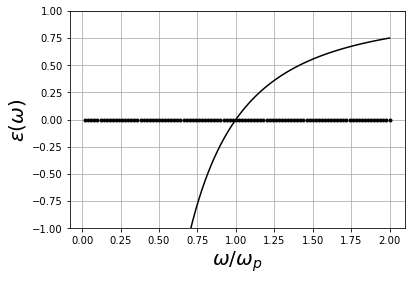
Para realizar la Fig. 1 de este paper, primeramente graficamos la funcion dielectrica con el siguiente programa
import numpy as np
import matplotlib.pyplot as plt
import math
import cmath
from scipy import linalg

c      = 3.0e8
wp     = 10        # eV
h_bar  = 6.58e-16
im     = complex(0,1)

wp     = wp/h_bar
gamma  = 0.0*wp

Nw   = 100
wi   = 0.0*wp
wf   = 2.0*wp
dw   = (wf-wi)/Nw
w    = np.zeros(Nw)
epsi = np.zeros(Nw,dtype=complex)

for iw in range(1,Nw+1):
  w[iw-1]     = wi+iw*dw
  epsi[iw-1]  = 1.0-(wp*wp)/(w[iw-1]*(w[iw-1]+im*gamma))
Luego graficamos con el codigo
plt.plot(w/wp,epsi.real,'-k',w/wp,epsi.imag,'.k')

plt.xlabel(r'$\omega/\omega_p$',fontsize=20)
plt.ylabel(r'$\varepsilon(\omega$)',fontsize=20)
#plt.xlim(0,0.5)
plt.ylim(-1,1)
plt.grid()
plt.show()
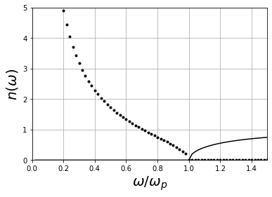
n=np.sqrt(epsi)

plt.plot(w/wp,n.real,'-k',w/wp,n.imag,'.k')

plt.xlabel(r'$\omega/\omega_p$',fontsize=20)
plt.ylabel(r'$n(\omega$)',fontsize=20)
plt.xlim(0,1.5)
plt.ylim(0,5)
plt.grid()
plt.show()
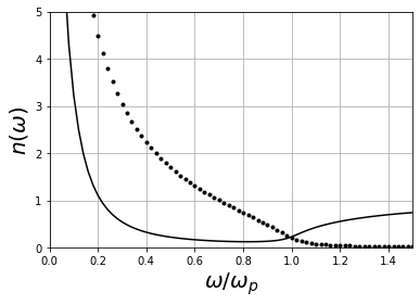
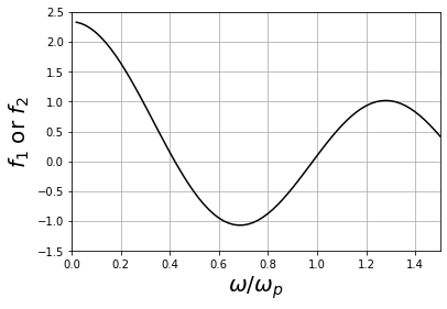
Para hacer el panel b de la figura 1 es necesario usar gamma=0.1wp, para tener
import numpy as np
import matplotlib.pyplot as plt
import math
import cmath
from scipy import linalg

c      = 3.0e8
wp     = 10        # eV
h_bar  = 6.58e-16
im     = complex(0,1)

d      = 100e-9
a      = 0.1*d
b      = d-a


wp     = wp/h_bar
gamma  = 0.00001*wp

Nw     = 100
wi     = 0.0*wp
wf     = 2.0*wp
dw     = (wf-wi)/Nw
w      = np.zeros(Nw)
epsi1  = np.zeros(Nw,dtype=complex)
n1     = np.zeros(Nw,dtype=complex)
aux10  = np.zeros(Nw,dtype=complex)

for iw in range(1,Nw+1):
  w[iw-1]     = wi+iw*dw
  epsi1[iw-1] = 1.0-(wp*wp)/(w[iw-1]*(w[iw-1]+im*gamma))
  n1[iw-1]    = cmath.sqrt(epsi1[iw-1])
  n2          = 1.0
  aux1 = cmath.cos(n1[iw-1]*(w[iw-1]/c)*a)*math.cos(n2*(w[iw-1]/c)*b)
  aux2 = 0.5*(n1[iw-1]/n2+n2/n1[iw-1])
  aux3 = cmath.sin(n1[iw-1]*(w[iw-1]/c)*a)*math.sin(n2*(w[iw-1]/c)*b)
  aux10[iw-1] = aux1-aux2*aux3
#  coseno[iw-1] = cmath.acos(aux4)/(2.0*math.pi)

plt.plot(w/wp,aux10.real,'-k')
plt.xlabel(r'$\omega/\omega_p$',fontsize=20)
plt.ylabel(r'$f_1$ or $f_2$',fontsize=20)
plt.xlim(0,1.5)
plt.ylim(-1.5,2.5)
plt.grid()
plt.show()
import numpy as np
import matplotlib.pyplot as plt
import math
import cmath
from scipy import linalg
c = 3.0e8
wp = 10 # eV
h_bar = 6.58e-16
im = complex(0,1)
d = 100e-9
a = 0.1*d
b = d-a
wp = wp/h_bar
gamma = 0.01*wp
Nw = 100
wi = 0.0*wp
wf = 2.0*wp
dw = (wf-wi)/Nw
w = np.zeros(Nw)
epsi1 = np.zeros(Nw,dtype=complex)
n1 = np.zeros(Nw,dtype=complex)
aux10 = np.zeros(Nw,dtype=complex)
for iw in range(1,Nw+1):
w[iw-1] = wi+iw*dw
epsi1[iw-1] = 1.0-(wp*wp)/(w[iw-1]*(w[iw-1]+im*gamma))
n1[iw-1] = cmath.sqrt(epsi1[iw-1])
n2 = 1.0
aux1 = cmath.cos(n1[iw-1]*(w[iw-1]/c)*a)*math.cos(n2*(w[iw-1]/c)*b)
aux2 = 0.5*(n1[iw-1]/n2+n2/n1[iw-1])
aux3 = cmath.sin(n1[iw-1]*(w[iw-1]/c)*a)*math.sin(n2*(w[iw-1]/c)*b)
aux10[iw-1] = aux1-aux2*aux3
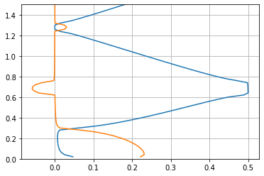
aux10[iw-1] = cmath.acos(aux10[iw-1])/(2.0*math.pi)
plt.plot(aux10.real,w/wp,aux10.imag,w/wp)
#plt.xlim(0,1.5)
plt.ylim(0,1.5)
plt.grid()
plt.show()
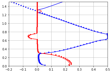
Comparacion con el metodo de estructura de bandas complejas
import numpy as np
import matplotlib.pyplot as plt
import math
import cmath
from scipy import linalg

c      = 3.0e8
wp     = 10        # eV
h_bar  = 6.58e-16
im     = complex(0,1)

d      = 100e-9
a      = 0.1*d
b      = d-a
f      = b/d


wp     = wp/h_bar
gamma  = 0.01*wp

Nw     = 100
wi     = 0.0*wp
wf     = 2.0*wp
dw     = (wf-wi)/Nw
w      = np.zeros(Nw)
epsi1  = np.zeros(Nw,dtype=complex)
n1     = np.zeros(Nw,dtype=complex)
aux10  = np.zeros(Nw,dtype=complex)
q0     = np.zeros(Nw,dtype=complex)
q1     = np.zeros(Nw,dtype=complex)
q2     = np.zeros(Nw,dtype=complex)
q3     = np.zeros(Nw,dtype=complex)

for iw in range(1,Nw+1):
  w[iw-1]     = wi+iw*dw
  epsi1[iw-1] = 1.0-(wp*wp)/(w[iw-1]*(w[iw-1]+im*gamma))
  n1[iw-1]    = cmath.sqrt(epsi1[iw-1])
  epsi2       = 1.0
  n2          = math.sqrt(epsi2)
  aux1 = cmath.cos(n1[iw-1]*(w[iw-1]/c)*a)*math.cos(n2*(w[iw-1]/c)*b)
  aux2 = 0.5*(n1[iw-1]/n2+n2/n1[iw-1])
  aux3 = cmath.sin(n1[iw-1]*(w[iw-1]/c)*a)*math.sin(n2*(w[iw-1]/c)*b)
  aux10[iw-1] = aux1-aux2*aux3
  aux10[iw-1] = cmath.acos(aux10[iw-1])/(2.0*math.pi)

  e_0   = epsi1[iw-1]+f*(epsi2-epsi1[iw-1])
  e_p1  = f*(epsi2-epsi1[iw-1])*(math.sin(math.pi*f)/(math.pi*f))
  e_m1  = f*(epsi2-epsi1[iw-1])*(math.sin(-math.pi*f)/(-math.pi*f))

  Om    = (w[iw-1]*d)/(2*math.pi*c)
  AA     = [[1,0],[0,1]]
  BB     = [[-2,0],[0,0]]
  CC     = [[1-Om*Om*e_0, -Om*Om*e_m1],
           [ -Om*Om*e_p1,-Om*Om*e_0]]
  ZZ     = [[0,0],[0,0]]
  II     = [[1,0],[0,1]]

  AAA    = [[CC[0][0],CC[0][1],BB[0][0],BB[0][1]],
            [CC[1][0],CC[1][1],BB[1][0],BB[1][1]],
            [ZZ[0][0],ZZ[0][1],II[0][0],II[0][1]],
            [ZZ[1][0],ZZ[1][1],II[1][0],II[1][1]]]


  BBB    = [[ZZ[0][0],ZZ[0][1],-AA[0][0],-AA[0][1]],
            [ZZ[1][0],ZZ[1][1],-AA[1][0],-AA[1][1]],
            [II[0][0],II[0][1], ZZ[0][0], ZZ[0][1]],
            [II[1][0],II[1][1], ZZ[1][0], ZZ[1][1]]]
  eigen,X       = linalg.eig(AAA,BBB)
  eigen.sort()
  q0[iw-1]       = eigen[0]
  q1[iw-1]       = eigen[1]
  q2[iw-1]       = eigen[2]
  q3[iw-1]       = eigen[3]

plt.plot(aux10.real,w/wp,'-b',aux10.imag,w/wp,'-r')
plt.plot(q1.real,w/wp,'.b',q1.imag,w/wp,'.r')
plt.xlim(-0.2,0.5)
plt.ylim(0,1.5)
plt.grid()
plt.show()