import numpy as np
from scipy.io.wavfile import write
import math
import matplotlib.pyplot as plt
## PARAMETROS DE LA SENIAL
amplitud = 32767 # Amplitud máxima (para 16-bit PCM)
fs = 44100 # Frecuencia de muestreo en Hz (común para audio de alta calidad)
ts = 1/fs
## PARAMETROS DE LA SENIAL
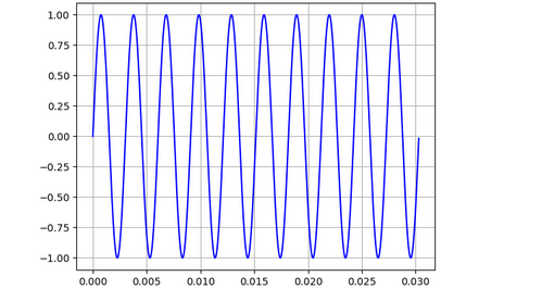
f0 = 330
t0 = 1/f0
ti = 0.0
tf = 10*t0
Nt = int((tf-ti)*fs)
t = np.zeros(Nt+1)
st = np.zeros(Nt+1)
for it in range(Nt+1):
t[it] = ti+it*ts
st[it] = math.sin(2.0*math.pi*f0*t[it])
plt.plot(t,st,'b')
plt.grid()
plt.show()
senal = amplitud*st
senal_int16 = np.int16(senal)
write("senal_sinusoidal.wav", fs, senal_int16)
print("Archivo WAV generado con éxito.")
import numpy as np
from scipy.io.wavfile import write
import math
import matplotlib.pyplot as plt
from scipy.fft import fft, fftfreq
## PARAMETROS DE LA SENIAL
amplitud = 32767 # Amplitud máxima (para 16-bit PCM)
fs = 44100 # Frecuencia de muestreo en Hz (común para audio de alta calidad)
ts = 1/fs
## PARAMETROS DE LA SENIAL
f0 = 330
t0 = 1/f0
ti = 0.0
tf = 10*t0
Nt = int((tf-ti)*fs)
t = np.zeros(Nt+1)
st = np.zeros(Nt+1)
for it in range(Nt+1):
t[it] = ti+it*ts
st[it] = math.sin(2.0*math.pi*f0*t[it])
fft_values = fft(st)
fft_freqs = fftfreq(len(fft_values), 1/fs)
# Graficar la señal original
plt.figure(figsize=(12, 6))
plt.subplot(2, 1, 1)
plt.plot(t, st, 'b')
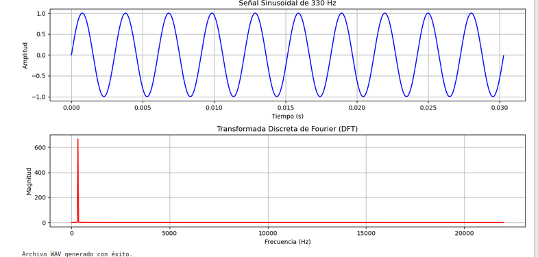
plt.title("Señal Sinusoidal de 330 Hz")
plt.xlabel("Tiempo (s)")
plt.ylabel("Amplitud")
plt.grid()
# Graficar la magnitud de la DFT
plt.subplot(2, 1, 2)
plt.plot(fft_freqs[:len(fft_values)//2], np.abs(fft_values)[:len(fft_values)//2], 'r')
plt.title("Transformada Discreta de Fourier (DFT)")
plt.xlabel("Frecuencia (Hz)")
plt.ylabel("Magnitud")
plt.grid()
plt.tight_layout()
plt.show()
senal = amplitud*st
senal_int16 = np.int16(senal)
write("senal_sinusoidal.wav", fs, senal_int16)
print("Archivo WAV generado con éxito.")
import numpy as np
from scipy.io.wavfile import write
import math
import matplotlib.pyplot as plt
from scipy.fft import fft, fftfreq
## PARAMETROS DE LA SENIAL
amplitud = 32767 # Amplitud máxima (para 16-bit PCM)
fs = 44100 # Frecuencia de muestreo en Hz (común para audio de alta calidad)
ts = 1/fs
## PARAMETROS DE LA SENIAL
f0 = 330
t0 = 1/f0
ti = 0.0
tf = 10*t0
Nt = int((tf-ti)*fs)
t = np.zeros(Nt+1)
st = np.zeros(Nt+1)
for it in range(Nt+1):
t[it] = ti+it*ts
st[it] = math.sin(2.0*math.pi*f0*t[it])
# Zero-padding: Agregar ceros para aumentar la resolución
n_padded = 20096 # Número de puntos para la DFT (aumenta la resolución)
signal_padded = np.pad(st, (0, n_padded - len(st)), 'constant')
# Calcular la DFT
fft_values = fft(signal_padded)
fft_freqs = fftfreq(len(fft_values), 1/fs)
# Graficar la señal original
plt.figure(figsize=(12, 6))
plt.subplot(2, 1, 1)
plt.plot(t, st, 'b')
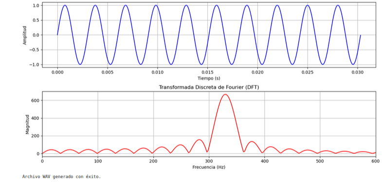
plt.title("Señal Sinusoidal de 330 Hz")
plt.xlabel("Tiempo (s)")
plt.ylabel("Amplitud")
plt.grid()
# Graficar la magnitud de la DFT
plt.subplot(2, 1, 2)
plt.plot(fft_freqs[:len(fft_values)//2], np.abs(fft_values)[:len(fft_values)//2], 'r')
plt.title("Transformada Discreta de Fourier (DFT)")
plt.xlabel("Frecuencia (Hz)")
plt.ylabel("Magnitud")
plt.xlim([0,600])
plt.grid()
plt.tight_layout()
plt.show()
senal = amplitud*st
senal_int16 = np.int16(senal)
write("senal_sinusoidal.wav", fs, senal_int16)
print("Archivo WAV generado con éxito.")