https://es.wikipedia.org/wiki/Ecuaci%C3%B3n_del_calor
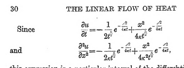
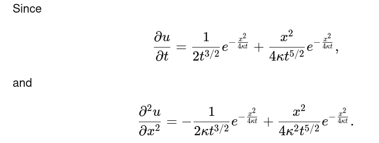
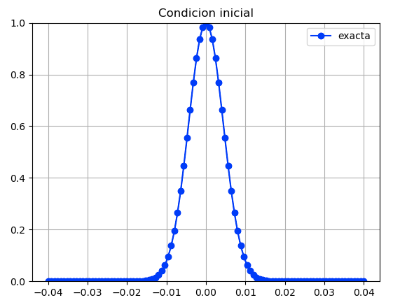
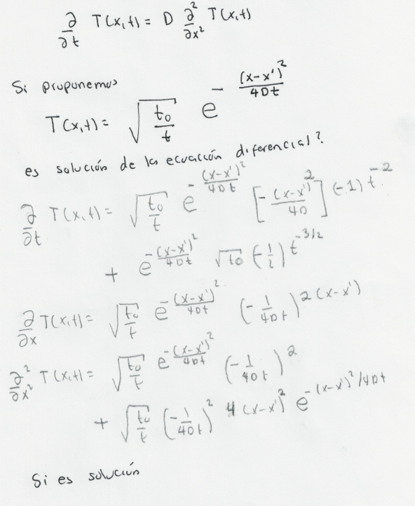
Analizemos una solucion tipica de la cuacion de calor en 1D descrita en el libro “Introduction To The Mathematical Theory Of The Conduction Of Heat In Solid” de Horatio Scott Carslaw.
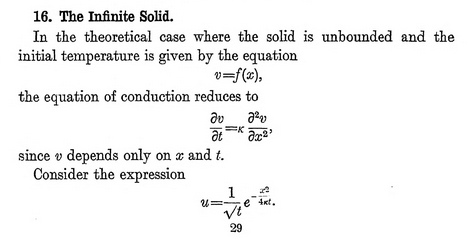
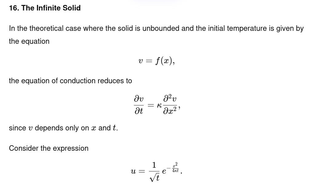
import numpy as np
import matplotlib.pyplot as plt
import math
import cmath
kappa_al  = 237.0;
rho_al    = 2698.4;
c_al      = 900.0;
D         = kappa_al/(rho_al*c_al);
Nx        = 100
xi        = -0.04;
xf        =  0.04;
dx        = (xf-xi)/Nx;
x         = np.zeros(Nx+1)
TTa       = np.zeros(Nx+1)
TTn       = np.zeros(Nx+1)
t0        = 0.1
Nt        = 500;
dt        = 0.2*(dx*dx)/(2.0*D);
t         = np.zeros(Nt+1)
#
it        = 0
t[it]     = t0
for ix in range(0,Nx+1):
  x[ix]  = xi+ix*dx
  TTa[ix]= math.sqrt(t0/t[it])*math.exp(-(x[ix]*x[ix])/(4.0*D*t[it]))
  TTn[ix]= TTa[ix]

plt.ylim(0,1)
plt.plot(x,TTa,'-ob',label='exacta')
plt.legend()
plt.grid()
plt.title("Condicion inicial")
plt.savefig("T_00{}.png".format(0))
plt.close()
for it in range(1,Nt+1):
  t[it]     = t0+it*dt
  for ix in range(1,Nx):
    TTa[ix]= math.sqrt(t0/t[it])*math.exp(-(x[ix]*x[ix])/(4.0*D*t[it]))
    TTn[ix]= TTn[ix] + ((D*dt)/(dx*dx))*(TTn[ix+1]-2.0*TTn[ix]+TTn[ix-1])
  plt.ylim(0,1)
  plt.plot(x,TTa,'-b',label='exacta')
  plt.plot(x,TTn,'or',label='FDTD')
  plt.title(f"t = {t[it]:.5f} s    paso = {it}/{Nt}")
  plt.legend()
  plt.grid()
  if it < 10:              plt.savefig("T_00{}.png".format(it))
  if it >= 10  and it<100: plt.savefig( "T_0{}.png".format(it))
  if it >= 100 and it<1000: plt.savefig(  "T_{}.png".format(it))
  plt.close()
import numpy as np
import matplotlib.pyplot as plt
import math
import cmath
kappa_al = 237.0;
rho_al = 2698.4;
c_al = 900.0;
D = kappa_al/(rho_al*c_al);
Nx = 100
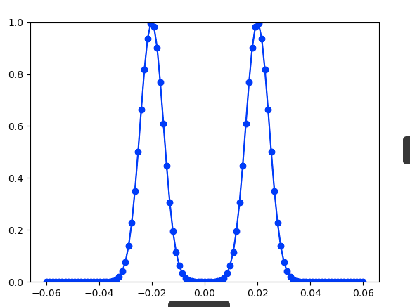
xi = -0.06;
xf = 0.06;
dx = (xf-xi)/Nx;
x = np.zeros(Nx+1)
TTa = np.zeros(Nx+1)
TTn = np.zeros(Nx+1)
t0 = 0.1
Nt = 500;
dt = 0.2*(dx*dx)/(2.0*D);
t = np.zeros(Nt+1)
#
it = 0
t[it] = t0
xp=0.02
for ix in range(0,Nx+1):
x[ix] = xi+ix*dx
aux1= math.sqrt(t0/t[it])*math.exp(-((x[ix]-xp)*(x[ix]-xp))/(4.0*D*t[it]))
aux2= math.sqrt(t0/t[it])*math.exp(-((x[ix]+xp)*(x[ix]+xp))/(4.0*D*t[it]))
TTa[ix]= aux1+aux2
TTn[ix]= TTa[ix]
plt.ylim(0,1)
plt.plot(x,TTa,'-ob')
plt.savefig("P_00{}.png".format(0))
plt.close()
for it in range(1,Nt+1):
t[it] = t0+it*dt
for ix in range(1,Nx):
# TTa[ix]= math.sqrt(t0/t[it])*math.exp(-(x[ix]*x[ix])/(4.0*D*t[it]))
aux1= math.sqrt(t0/t[it])*math.exp(-((x[ix]-xp)*(x[ix]-xp))/(4.0*D*t[it]))
aux2= math.sqrt(t0/t[it])*math.exp(-((x[ix]+xp)*(x[ix]+xp))/(4.0*D*t[it]))
TTa[ix]= aux1+aux2
TTn[ix]= TTn[ix] + ((D*dt)/(dx*dx))*(TTn[ix+1]-2.0*TTn[ix]+TTn[ix-1])
plt.ylim(0,1)
plt.plot(x,TTa,'-b',label='exacta')
plt.plot(x,TTn,'or',label='FDTD')
plt.title(f"t = {t[it]:.5f} s paso = {it}/{Nt}")
plt.legend()
plt.grid()
if it < 10: plt.savefig("P_00{}.png".format(it))
if it >= 10 and it<100: plt.savefig( "P_0{}.png".format(it))
if it >= 100 and it<1000: plt.savefig( "P_{}.png".format(it))
plt.close()
#plt.savefig("T_00{}.png".format(0))
#plt.close()
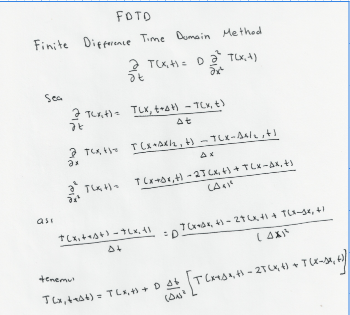
Que es el FDTD?
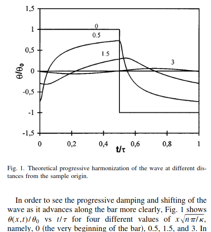
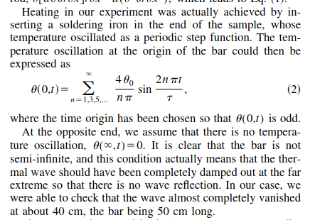
?Que son ondas termicas?
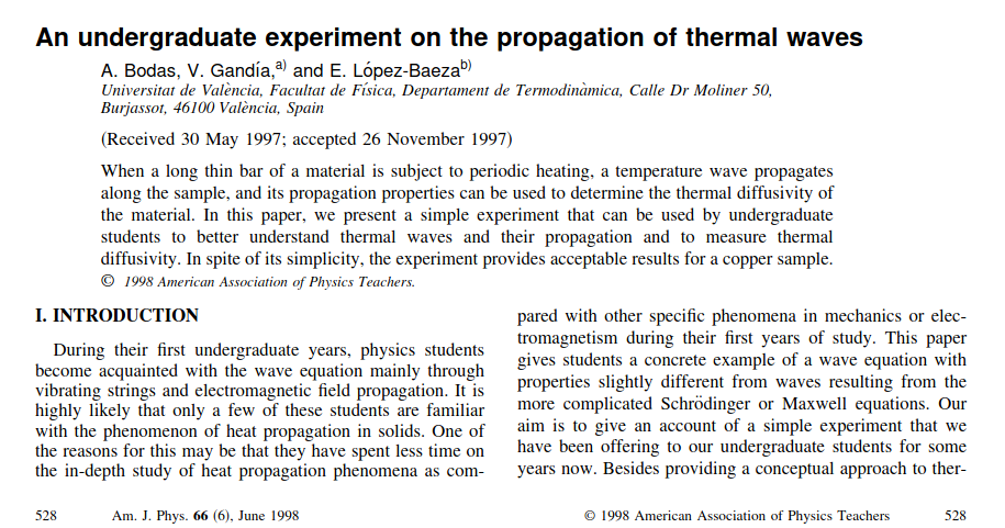
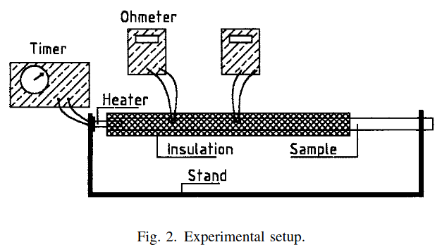
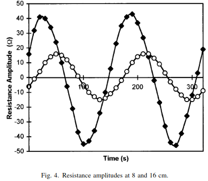
El experimento de Anwar