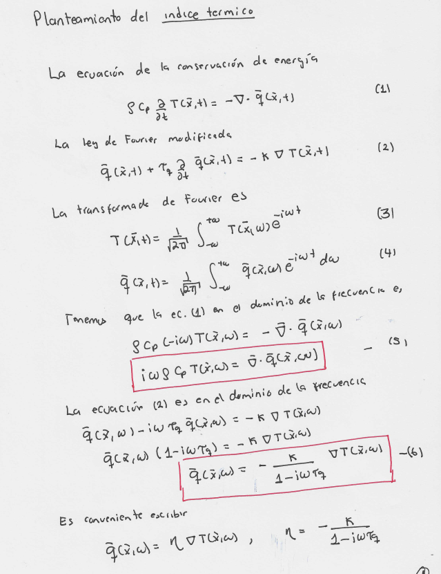
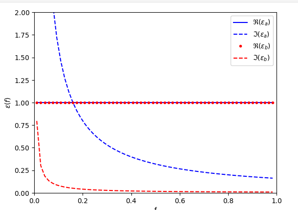
Analisis del medio de los medios dermis y stratum
La funcion dielectrica es
import numpy as np
import cmath
import math
import matplotlib.pyplot as plt
im = complex(0.0,1.0)
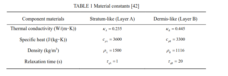
# Stratum
ka = 0.235
ca = 3600
ra = 1500
ta = 1
# Dermis
kb = 0.445
cb = 3300
rb = 1116
tb = 20
ea = np.zeros(Nf,dtype=complex)
Nf = 60
fi = 0.01 # Hz
ff = 1.0 # Hz
df = (ff-fi)/Nf
f = np.zeros(Nf)
ea = np.zeros(Nf,dtype=complex)
eb = np.zeros(Nf,dtype=complex)
for ic in range(Nf):
f[ic]=fi+ic*df
w = 2.0*math.pi*f[ic]
ea[ic] = 1.0 + im/(w*ta)
eb[ic] = 1.0 + im/(w*tb)
plt.plot(f,ea.real,'-b',label=r'$\Re(\varepsilon_a)$')
plt.plot(f,ea.imag,'--b',label=r'$\Im(\varepsilon_a)$')
plt.plot(f,eb.real,'.r',label=r'$\Re(\varepsilon_b)$')
plt.plot(f,eb.imag,'--r',label=r'$\Im(\varepsilon_b)$')
plt.ylim([0,2])
plt.xlim([0,1])
plt.xlabel('f')
plt.ylabel(r'$\varepsilon(f)$')
plt.legend()
plt.show()
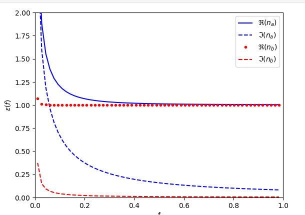
Ahora graficamos el indice
import numpy as np
import cmath
import math
import matplotlib.pyplot as plt
im = complex(0.0,1.0)
# Stratum
ka = 0.235
ca = 3600
ra = 1500
ta = 1
Cca = math.sqrt(ka/(ca*ra*ta))
# Dermis
kb = 0.445
cb = 3300
rb = 1116
tb = 20
Ccb = math.sqrt(kb/(cb*rb*tb))
Nf = 60
fi = 0.01 # Hz
ff = 1.0 # Hz
df = (ff-fi)/Nf
f = np.zeros(Nf)
ea = np.zeros(Nf,dtype=complex)
eb = np.zeros(Nf,dtype=complex)
na = np.zeros(Nf,dtype=complex)
nb = np.zeros(Nf,dtype=complex)
gamma_a = np.zeros(Nf,dtype=complex)
gamma_b = np.zeros(Nf,dtype=complex)
etaa = np.zeros(Nf,dtype=complex)
etab = np.zeros(Nf,dtype=complex)
for ic in range(Nf):
f[ic]=fi+ic*df
w = 2.0*math.pi*f[ic]
ea[ic] = 1.0 + im/(w*ta)
eb[ic] = 1.0 + im/(w*tb)
na[ic] = cmath.sqrt(ea[ic])
nb[ic] = cmath.sqrt(eb[ic])
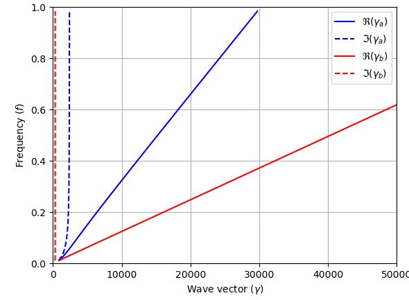
gamma_a[ic] = (w/Cca)*na[ic]
gamma_b[ic] = (w/Ccb)*nb[ic]
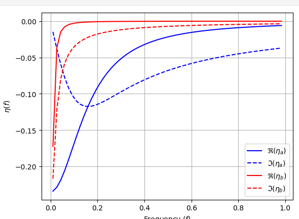
etaa[ic] = -ka/(1-im*w*ta)
etab[ic] = -kb/(1-im*w*tb)
####################################
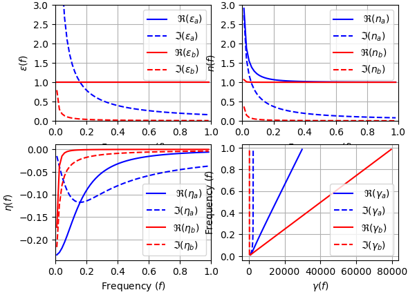
plt.subplot(2, 2, 1)
plt.plot(f,ea.real,'-b',label=r' $\Re(\varepsilon_a)$')
plt.plot(f,ea.imag,'--b',label=r'$\Im(\varepsilon_a)$')
plt.plot(f,eb.real,'-r',label=r'$\Re(\varepsilon_b)$')
plt.plot(f,eb.imag,'--r',label=r'$\Im(\varepsilon_b)$')
plt.xlim([0,1])
plt.ylim([0,3])
plt.ylabel(r'$\varepsilon(f)$')
plt.xlabel(r'Frequency $(f)$')
plt.grid()
plt.legend()
####################################
plt.subplot(2, 2, 2)
plt.plot(f,na.real,'-b',label=r' $\Re(n_a)$')
plt.plot(f,na.imag,'--b',label=r'$\Im(n_a)$')
plt.plot(f,nb.real,'-r',label=r'$\Re(n_b)$')
plt.plot(f,nb.imag,'--r',label=r'$\Im(n_b)$')
plt.xlim([0,1])
plt.ylim([0,3])
plt.ylabel(r'$n(f)$')
plt.xlabel(r'Frequency $(f)$')
plt.grid()
plt.legend()
####################################
plt.subplot(2, 2, 3)
plt.plot(f,etaa.real,'-b',label=r' $\Re(\eta_a)$')
plt.plot(f,etaa.imag,'--b',label=r'$\Im(\eta_a)$')
plt.plot(f,etab.real,'-r',label=r'$\Re(\eta_b)$')
plt.plot(f,etab.imag,'--r',label=r'$\Im(\eta_b)$')
plt.xlim([0,1])
#plt.ylim([0,3])
plt.ylabel(r'$\eta(f)$')
plt.xlabel(r'Frequency $(f)$')
plt.grid()
plt.legend()
####################################
plt.subplot(2, 2, 4)
plt.plot(gamma_a.real,f,'-b',label=r' $\Re(\gamma_a)$')
plt.plot(gamma_a.imag,f,'--b',label=r'$\Im(\gamma_a)$')
plt.plot(gamma_b.real,f,'-r',label=r'$\Re(\gamma_b)$')
plt.plot(gamma_b.imag,f,'--r',label=r'$\Im(\gamma_b)$')
#plt.xlim([0,1])
#plt.ylim([0,3])
plt.xlabel(r'$\gamma(f)$')
plt.ylabel(r'Frequency $(f)$')
plt.grid()
plt.legend()
plt.show()

import numpy as np
import cmath
import math
import matplotlib.pyplot as plt
im = complex(0.0,1.0)
# Stratum
ka = 0.235
ca = 3600
ra = 1500
ta = 1
Cca = math.sqrt(ka/(ca*ra*ta))
# Dermis
kb = 0.445
cb = 3300
rb = 1116
tb = 20
Ccb = math.sqrt(kb/(cb*rb*tb))
Nf = 60
fi = 0.01 # Hz
ff = 1.0 # Hz
df = (ff-fi)/Nf
f = np.zeros(Nf)
ea = np.zeros(Nf,dtype=complex)
eb = np.zeros(Nf,dtype=complex)
na = np.zeros(Nf,dtype=complex)
nb = np.zeros(Nf,dtype=complex)
gamma_a = np.zeros(Nf,dtype=complex)
gamma_b = np.zeros(Nf,dtype=complex)
etaa = np.zeros(Nf,dtype=complex)
etab = np.zeros(Nf,dtype=complex)
f=4.0
w = 2.0*math.pi*f
ea = 1.0 + im/(w*ta)
eb = 1.0 + im/(w*tb)
na = cmath.sqrt(ea)
nb = cmath.sqrt(eb)
gamma_a = (w/Cca)*na
gamma_b = (w/Ccb)*nb
Nx = 1000
xi = 0.00
xf = 0.001
dx = (xf-xi)/Nx
xp = np.zeros(Nx)
xm = np.zeros(Nx)
Tap = np.zeros(Nx,dtype=complex)
Tam = np.zeros(Nx,dtype=complex)
Tbp = np.zeros(Nx,dtype=complex)
Tbm = np.zeros(Nx,dtype=complex)
for ix in range(Nx):
xp[ix] = xi + ix*dx
Tap[ix] = cmath.exp(+im*gamma_a*xp[ix])
Tbp[ix] = cmath.exp(+im*gamma_b*xp[ix])
xi = -0.001
xf = 0.000
dx = (xf-xi)/Nx
for ix in range(Nx):
xm[ix] = xi + ix*dx
Tam[ix] = cmath.exp(-im*gamma_a*xm[ix])
Tbm[ix] = cmath.exp(-im*gamma_b*xm[ix])
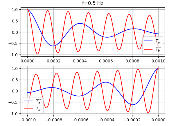
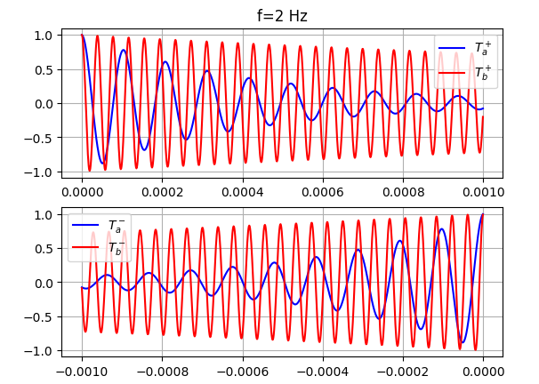
plt.subplot(2,1,1)
plt.grid()
plt.title('f=4 Hz')
plt.plot(xp,Tap.real,'-b',label=r'$T_a^+$')
plt.plot(xp,Tbp.real,'-r',label=r'$T_b^+$')
plt.legend()
plt.subplot(2,1,2)
plt.grid()
plt.plot(xm,Tam.real,'-b',label=r'$T_a^-$')
plt.plot(xm,Tbm.real,'-r',label=r'$T_b^-$')
plt.legend()
plt.show()