import meep as mp
import numpy as  np
import math
from matplotlib import pyplot as plt

############## -> H
NH = 220
Hi = 0.0
Hf = 11
dH = (Hf-Hi)/(NH)
HV =  np.zeros(NH)
maxV = np.zeros(NH)
QQxV = np.zeros(NH)
maxV = np.zeros(NH)
############# <- H

############# -> FT
i_0=500
i_I=800
I=i_I-i_0
Qx_i=0.01
Qx_f=1.0
NQx=100
dQx=(Qx_f-Qx_i)/NQx
EQx=np.zeros(NQx)
QxV=np.zeros(NQx)
mapaFT=np.zeros((NH,NQx))
############ <- FT


for iH in range(NH):
 H = Hi+iH*dH
 HV[iH] = H
 print(iH,H)

############################################### -> meep
 L = 40
 t_until=400
 cell = mp.Vector3(2*L, L, 0)
 geometry = [mp.Block(mp.Vector3(L,  1, mp.inf),center=mp.Vector3(-L/2,-H/2),material=mp.Medium(epsilon=3.6*3.6),e1=[1.0, 0.0],e2=[0.0, 1.0]),
             mp.Block(mp.Vector3(1,H+1, mp.inf),center=mp.Vector3(   0,   0),material=mp.Medium(epsilon=3.6*3.6),e1=[1.0, 0.0],e2=[0.0, 1.0]),
             mp.Block(mp.Vector3(L,  1, mp.inf),center=mp.Vector3(+L/2,+H/2),material=mp.Medium(epsilon=3.6*3.6),e1=[1.0, 0.0],e2=[0.0, 1.0])]
 sources = [mp.Source(mp.ContinuousSource(frequency=0.1), component=mp.Ez, center=mp.Vector3(-L+2, -H/2))]
 pml_layers = [mp.PML(1.0)]
 resolution = 10
 sim = mp.Simulation(cell_size=cell,boundary_layers=pml_layers,geometry=geometry,sources=sources,resolution=resolution,)
 print('----------------- H = ',H)
 plt.figure(dpi=100)
 sim.plot2D()
 plt.savefig('a'+str(H)+'.png')
 plt.show()
 sim.run(until=t_until)
 plt.figure(dpi=100)
 sim.plot2D(fields=mp.Ez)
 plt.savefig('b'+str(H)+'.png')
 plt.show()
 eps_data = sim.get_array(center=mp.Vector3(), size=cell, component=mp.Dielectric)
 ez_data = sim.get_array(center=mp.Vector3(), size=cell, component=mp.Ez)
 plt.imshow(eps_data)
 plt.savefig('c'+str(H)+'.png')
 plt.show()
 plt.imshow(ez_data)
 plt.savefig('d'+str(H)+'.png')
 plt.show()
 plt.plot(ez_data[:,int((L/2+H/2)*10)])
 plt.savefig('e'+str(H)+'.png')
 plt.show()
################################################## <- meep


################################################## -> FT
 for iQx in range(NQx):
  Qx = Qx_i+iQx*dQx
  QxV[iQx]=Qx
  Exr=0
  Exi=0
  for i in range(I):
   Exr=Exr+ez_data[i_0+i,int((L/2+H/2)*10)]*math.cos(2.0*math.pi*Qx*((i_0+i)/resolution))
   Exi=Exi+ez_data[i_0+i,int((L/2+H/2)*10)]*math.sin(2.0*math.pi*Qx*((i_0+i)/resolution))
  EQx[iQx] = math.sqrt(Exr*Exr+Exi*Exi)
  mapaFT[iH,iQx]=EQx[iQx]
 plt.plot(QxV,EQx)
 plt.savefig('f'+str(H)+'.png')
 plt.show()
 maxV[iH] =  np.max(EQx)
 el_indice = np.argmax(EQx)
 QQxV[iH] = QxV[el_indice]
#################################################### <- FT
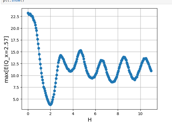
plt.plot(HV,maxV,'-o')


plt.xlabel('H', fontsize=14)
plt.ylabel('max[E(Q_x=2.57]', fontsize=14)


# Mostrar la gráfica
plt.grid()
plt.show()