new.jmanza@gmail.com – Página 3 – Jesus Manzanares Martinez

import meep as mp
import numpy as  np
import math
from matplotlib import pyplot as plt

############## -> H
NH = 220
Hi = 0.0
Hf = 11
dH = (Hf-Hi)/(NH)
HV =  np.zeros(NH)
maxV = np.zeros(NH)
QQxV = np.zeros(NH)
maxV = np.zeros(NH)
############# <- H

############# -> FT
i_0=500
i_I=800
I=i_I-i_0
Qx_i=0.01
Qx_f=1.0
NQx=100
dQx=(Qx_f-Qx_i)/NQx
EQx=np.zeros(NQx)
QxV=np.zeros(NQx)
mapaFT=np.zeros((NH,NQx))
############ <- FT


for iH in range(NH):
 H = Hi+iH*dH
 HV[iH] = H
 print(iH,H)
    
############################################### -> meep 
 L = 40
 t_until=400
 cell = mp.Vector3(2*L, L, 0)
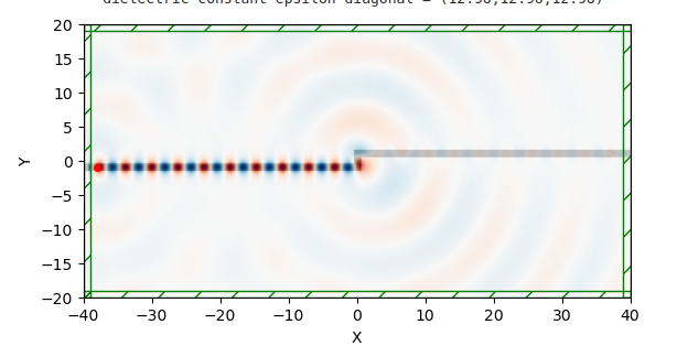
 geometry = [mp.Block(mp.Vector3(L,  1, mp.inf),center=mp.Vector3(-L/2,-H/2),material=mp.Medium(epsilon=3.6*3.6),e1=[1.0, 0.0],e2=[0.0, 1.0]),
             mp.Block(mp.Vector3(1,H+1, mp.inf),center=mp.Vector3(   0,   0),material=mp.Medium(epsilon=3.6*3.6),e1=[1.0, 0.0],e2=[0.0, 1.0]),
             mp.Block(mp.Vector3(L,  1, mp.inf),center=mp.Vector3(+L/2,+H/2),material=mp.Medium(epsilon=3.6*3.6),e1=[1.0, 0.0],e2=[0.0, 1.0])]
 sources = [mp.Source(mp.ContinuousSource(frequency=0.1), component=mp.Ez, center=mp.Vector3(-L+2, -H/2))]
 pml_layers = [mp.PML(1.0)]
 resolution = 10
 sim = mp.Simulation(cell_size=cell,boundary_layers=pml_layers,geometry=geometry,sources=sources,resolution=resolution,)
 print('----------------- H = ',H)
 plt.figure(dpi=100)
 sim.plot2D()
 plt.savefig('a'+str(H)+'.png')
 plt.show()
 sim.run(until=t_until)
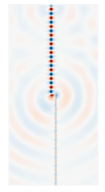
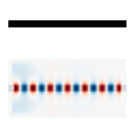
 plt.figure(dpi=100)
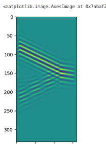
 sim.plot2D(fields=mp.Ez)
 plt.savefig('b'+str(H)+'.png')
 plt.show()
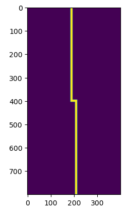
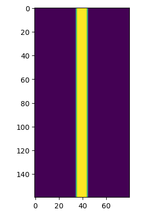
 eps_data = sim.get_array(center=mp.Vector3(), size=cell, component=mp.Dielectric)
 ez_data = sim.get_array(center=mp.Vector3(), size=cell, component=mp.Ez)
 plt.imshow(eps_data)
 plt.savefig('c'+str(H)+'.png')
 plt.show()
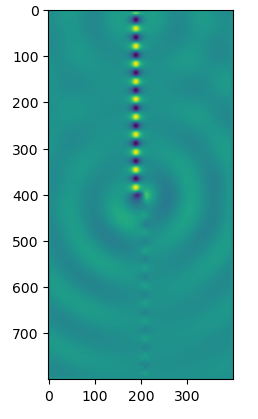
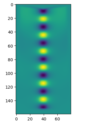
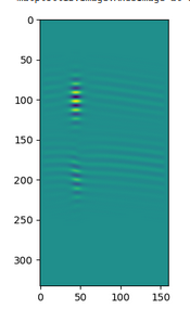
 plt.imshow(ez_data)
 plt.savefig('d'+str(H)+'.png')
 plt.show()
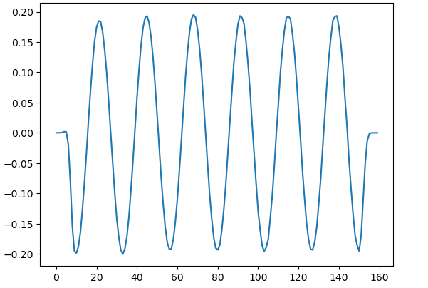
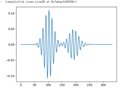
 plt.plot(ez_data[:,int((L/2+H/2)*10)])
 plt.savefig('e'+str(H)+'.png')
 plt.show()
################################################## <- meep


################################################## -> FT
 for iQx in range(NQx):
  Qx = Qx_i+iQx*dQx
  QxV[iQx]=Qx
  Exr=0
  Exi=0
  for i in range(I):
   Exr=Exr+ez_data[i_0+i,int((L/2+H/2)*10)]*math.cos(2.0*math.pi*Qx*((i_0+i)/resolution))
   Exi=Exi+ez_data[i_0+i,int((L/2+H/2)*10)]*math.sin(2.0*math.pi*Qx*((i_0+i)/resolution))
  EQx[iQx] = math.sqrt(Exr*Exr+Exi*Exi)  
  mapaFT[iH,iQx]=EQx[iQx]
 plt.plot(QxV,EQx)
 plt.savefig('f'+str(H)+'.png')
 plt.show()
 maxV[iH] =  np.max(EQx)
 el_indice = np.argmax(EQx)
 QQxV[iH] = QxV[el_indice]
#################################################### <- FT

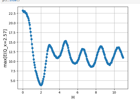
plt.plot(HV,maxV,'-o')


plt.xlabel('H', fontsize=14)
plt.ylabel('max[E(Q_x=2.57]', fontsize=14)


# Mostrar la gráfica
plt.grid()
plt.show()

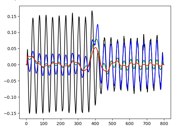
Entendiendo las tripas del meep: doblez2 y la FT

import meep as mp

L = 40
H = 1
t_until=400
cell = mp.Vector3(2*L, L, 0)
geometry = [mp.Block(mp.Vector3(L,  1, mp.inf),center=mp.Vector3(-L/2,-H/2),material=mp.Medium(epsilon=3.6*3.6),e1=[1.0, 0.0],e2=[0.0, 1.0]),
            mp.Block(mp.Vector3(1,H+1, mp.inf),center=mp.Vector3(   0,   0),material=mp.Medium(epsilon=3.6*3.6),e1=[1.0, 0.0],e2=[0.0, 1.0]),
            mp.Block(mp.Vector3(L,  1, mp.inf),center=mp.Vector3(+L/2,+H/2),material=mp.Medium(epsilon=3.6*3.6),e1=[1.0, 0.0],e2=[0.0, 1.0])]
sources = [mp.Source(mp.ContinuousSource(frequency=0.1), component=mp.Ez, center=mp.Vector3(-L+2, -H/2))]
pml_layers = [mp.PML(1.0)]
resolution = 10
sim = mp.Simulation(cell_size=cell,boundary_layers=pml_layers,geometry=geometry,sources=sources,resolution=resolution,)


from matplotlib import pyplot as plt
plt.figure(dpi=100)
sim.plot2D()
plt.show()

sim.run(until=t_until)
plt.figure(dpi=100)
sim.plot2D(fields=mp.Ez)
plt.show()

eps_data = sim.get_array(center=mp.Vector3(), size=cell, component=mp.Dielectric)
ez_data = sim.get_array(center=mp.Vector3(), size=cell, component=mp.Ez)

print(ez_data.shape)
plt.imshow(ez_data)

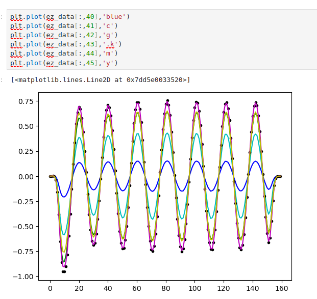
plt.plot(ez_data[:,200],'-k')
plt.plot(ez_data[:,210],'-b')
plt.plot(ez_data[:,220],'-g')
plt.plot(ez_data[:,230],'-r')

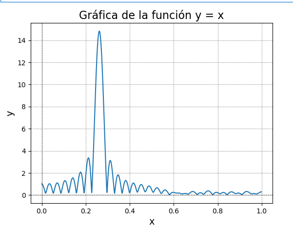
import numpy as np
import math

############ FT
i_0=500
i_I=800
I=i_I-i_0
Qx_i=0.0
Qx_f=1.0
NQx=1000
dQx=(Qx_f-Qx_i)/NQx
EQx=np.zeros(NQx)
QxV=np.zeros(NQx)
############# FT
for ic in range(NQx):
  Qx = Qx_i+ic*dQx
  QxV[ic]=Qx
  Exr=0
  Exi=0
  for i in range(I):
   Exr=Exr+ez_data[i_0+i,int((L/2+H/2)*10)]*math.cos(2.0*math.pi*Qx*(i_0+i)/resolution)
   Exi=Exi+ez_data[i_0+i,int((L/2+H/2)*10)]*math.sin(2.0*math.pi*Qx*(i_0+i)/resolution)
  EQx[ic] = math.sqrt(Exr*Exr+Exi*Exi)

plt.plot(QxV,EQx)



# Graficar


# Personalización de la gráfica
plt.title('Gráfica de la función y = x', fontsize=16)
plt.xlabel('x', fontsize=14)
plt.ylabel('y', fontsize=14)
plt.axhline(0, color='black',linewidth=0.5, ls='--')  # Línea horizontal en y=0
plt.axvline(0, color='black',linewidth=0.5, ls='--')  # Línea vertical en x=0
plt.grid(color = 'gray', linestyle = '--', linewidth = 0.5)
# Mostrar la gráfica
plt.show()

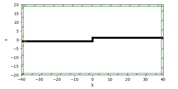
Entiendo las tripas del meep: doblez

import meep as mp
L = 40
H = 2
t_until=400
cell = mp.Vector3(2*L, L, 0)
geometry = [mp.Block(mp.Vector3(L,  1, mp.inf),center=mp.Vector3(-L/2,-H/2),material=mp.Medium(epsilon=3.6*3.6),e1=[1.0, 0.0],e2=[0.0, 1.0]),
            mp.Block(mp.Vector3(1,H+1, mp.inf),center=mp.Vector3(   0,   0),material=mp.Medium(epsilon=3.6*3.6),e1=[1.0, 0.0],e2=[0.0, 1.0]),
            mp.Block(mp.Vector3(L,  1, mp.inf),center=mp.Vector3(+L/2,+H/2),material=mp.Medium(epsilon=3.6*3.6),e1=[1.0, 0.0],e2=[0.0, 1.0])]
sources = [mp.Source(mp.ContinuousSource(frequency=0.1), component=mp.Ez, center=mp.Vector3(-L+2, -H/2))]
pml_layers = [mp.PML(1.0)]
resolution = 10
sim = mp.Simulation(cell_size=cell,boundary_layers=pml_layers,geometry=geometry,sources=sources,resolution=resolution,)

from matplotlib import pyplot as plt
plt.figure(dpi=100)
sim.plot2D()
plt.savefig('books_read'+str(H)+'.png')
plt.show()

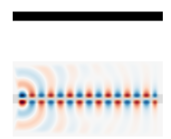
sim.run(until=t_until)
plt.figure(dpi=100)
sim.plot2D(fields=mp.Ez)
plt.show()

eps_data = sim.get_array(center=mp.Vector3(), size=cell, component=mp.Dielectric)
ez_data = sim.get_array(center=mp.Vector3(), size=cell, component=mp.Ez)
plt.figure()
plt.imshow(eps_data, interpolation='spline36', cmap='binary')
plt.imshow(ez_data, interpolation='spline36', cmap='RdBu', alpha=0.9)
plt.axis('off')
plt.show()

plt.imshow(ez_data)

plt.imshow(eps_data)

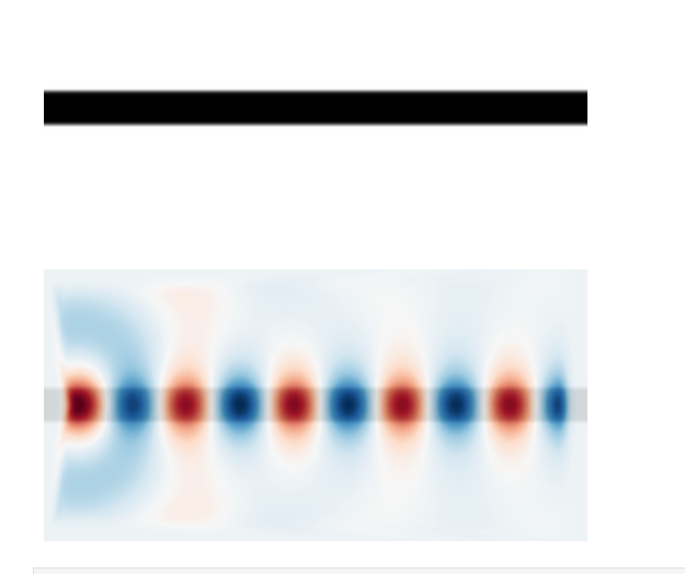
La guia recta

# From the Meep tutorial: plotting permittivity and fields of a straight waveguide
import meep as mp

cell = mp.Vector3(16, 8, 0)

geometry = [
    mp.Block(
        mp.Vector3(mp.inf, 1, mp.inf),
        center=mp.Vector3(),
        material=mp.Medium(epsilon=12),
    )
]

sources = [
    mp.Source(
        mp.ContinuousSource(frequency=0.15), component=mp.Ez, center=mp.Vector3(-7, 0)
    )
]

pml_layers = [mp.PML(1.0)]

resolution = 10

sim = mp.Simulation(
    cell_size=cell,
    boundary_layers=pml_layers,
    geometry=geometry,
    sources=sources,
    resolution=resolution,
)

sim.run(until=200)

Ahi el programa corre, para visualizar tenemos

import matplotlib.pyplot as plt
import numpy as np

eps_data = sim.get_array(center=mp.Vector3(), size=cell, component=mp.Dielectric)
plt.figure()
plt.imshow(eps_data.transpose(), interpolation="spline36", cmap="binary")
plt.axis("off")
plt.show()

ez_data = sim.get_array(center=mp.Vector3(), size=cell, component=mp.Ez)
plt.figure()
plt.imshow(eps_data.transpose(), interpolation="spline36", cmap="binary")
plt.imshow(ez_data.transpose(), interpolation="spline36", cmap="RdBu", alpha=0.9)
plt.axis("off")
plt.show()

Es muy interesante darse cuenta de que ya tenemos los datos de la funcion dielectrica en python y los podemos visualizar haciendo

plt.imshow(eps_data)

plt.imshow(ez_data)

plt.plot(ez_data[:,40])

Vamos a entender la relacion de dispersion

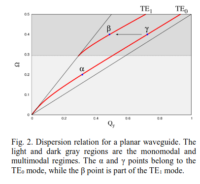
Este paper esta enhttps://www.google.com/url?sa=t&source=web&rct=j&opi=89978449&url=https://journals.riverpublishers.com/index.php/ACES/article/download/10289/8605/32011&ved=2ahUKEwjx0ZuEy8WLAxWjEEQIHdd_HiIQFnoECBIQAQ&usg=AOvVaw2g6KH89R-yyESrphePaN3H

Esta es una guia de $n_h=2$ en aire ( $n_l=1$ ).

import meep as mp
cell = mp.Vector3(16, 8, 0)
geometry = [mp.Block(mp.Vector3(mp.inf, 1, mp.inf),center=mp.Vector3(),material=mp.Medium(epsilon=4),)]
sources = [mp.Source(mp.ContinuousSource(frequency=0.2), component=mp.Ez, center=mp.Vector3(-7, 0))]
pml_layers = [mp.PML(1.0)]
resolution = 10
sim = mp.Simulation(cell_size=cell,boundary_layers=pml_layers,geometry=geometry,sources=sources,resolution=resolution,)
sim.run(until=200)

import matplotlib.pyplot as plt
import numpy as np

eps_data = sim.get_array(center=mp.Vector3(), size=cell, component=mp.Dielectric)
plt.figure()
plt.imshow(eps_data.transpose(), interpolation="spline36", cmap="binary")
plt.axis("off")
plt.show()

ez_data = sim.get_array(center=mp.Vector3(), size=cell, component=mp.Ez)
plt.figure()
plt.imshow(eps_data.transpose(), interpolation="spline36", cmap="binary")
plt.imshow(ez_data.transpose(), interpolation="spline36", cmap="RdBu", alpha=0.9)
plt.axis("off")
plt.show()

plt.plot(ez_data[:,40])

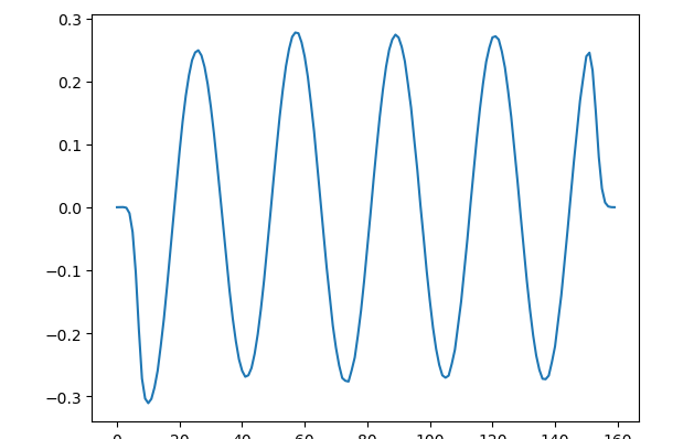
Para el modo en $|Omega=0.2$ tenemos que $Q_y=0.32$ , considerando que

$Q_y=\frac{k_yd}{2\pi}$

$Q_y=\frac{d}{\lambda_m}$

$\lambda_m = \frac{Q_y}{d}$

Para el caso de $Q_y=0.32$ tenemos $\lambda_m=(1/0.32)d=3.125 d$

Para poder medir la distancia entre valle y valle (o cresta y cresta), hacemos

f = open("python.dat","w")
for i in range(ez_data.shape[0]):
 print(i,ez_data[i,40])
 f.write(str(i/10.0)+" "+str(ez_data[i,40])+"\n")
f.close()

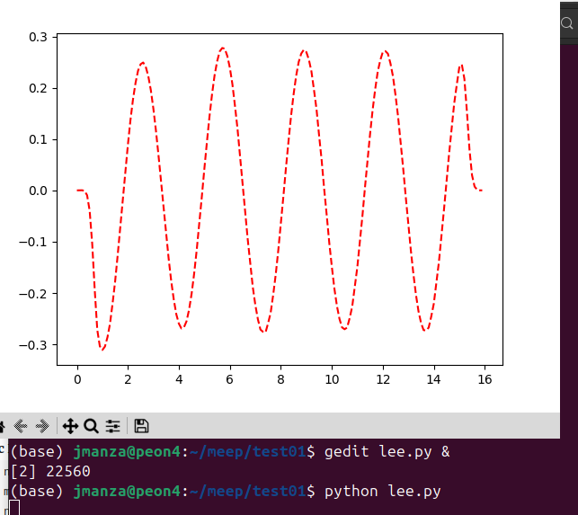
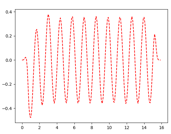
El siguiente codigo se llama lee.py y se corre en el sistema operativo para que se genere una grafica en donde con el mouse, se pueda medir las distancias

import numpy  as np
import matplotlib.pyplot as plt
data = np.loadtxt('python.dat')
x = data[:, 0]
y = data[:, 1]
plt.plot(x, y,'r--')
plt.show()

Cuando $\Omega=0.4$ , tenemos $Q_y=0.72$ , nos sale $\lambda = 1.38$ la longitud de onda, que e slo que vemos

Podemos generar el segundo modo

# From the Meep tutorial: plotting permittivity and fields of a straight waveguide
import meep as mp
cell = mp.Vector3(16, 8, 0)
geometry = [mp.Block(mp.Vector3(mp.inf, 1, mp.inf),center=mp.Vector3(),material=mp.Medium(epsilon=4),)]
sources = [mp.Source(mp.ContinuousSource(frequency=0.4), component=mp.Ez, center=mp.Vector3(-7,  0.4),amplitude=+1.0),
           mp.Source(mp.ContinuousSource(frequency=0.4), component=mp.Ez, center=mp.Vector3(-7, -0.4),amplitude=-1.0)]
pml_layers = [mp.PML(1.0)]
resolution = 10
sim = mp.Simulation(cell_size=cell,boundary_layers=pml_layers,geometry=geometry,sources=sources,resolution=resolution,)
sim.run(until=200)

import matplotlib.pyplot as plt
import numpy as np

eps_data = sim.get_array(center=mp.Vector3(), size=cell, component=mp.Dielectric)
plt.figure()
plt.imshow(eps_data.transpose(), interpolation="spline36", cmap="binary")
plt.axis("off")
plt.show()

ez_data = sim.get_array(center=mp.Vector3(), size=cell, component=mp.Ez)
plt.figure()
plt.imshow(eps_data.transpose(), interpolation="spline36", cmap="binary")
plt.imshow(ez_data.transpose(), interpolation="spline36", cmap="RdBu", alpha=0.9)
plt.axis("off")
plt.show()

Podemos checar que la maxima amplitud NO esta en el centro

eje temporal

# From the Meep tutorial: plotting permittivity and fields of a straight waveguide
import meep as mp
cell     = mp.Vector3(10, 10, 0)
geometry = [mp.Block(mp.Vector3(0.1, 0.1, mp.inf),center=mp.Vector3(4,4),material=mp.Medium(epsilon=1.1),)]
sources = [mp.Source(mp.ContinuousSource(frequency=0.8), component=mp.Ez, center=mp.Vector3(0, 0))]
pml_layers = [mp.PML(1.0)]
resolution = 10
sim = mp.Simulation(cell_size=cell,boundary_layers=pml_layers,geometry=geometry,sources=sources,resolution=resolution,)
sim.run(mp.at_beginning(mp.output_epsilon),mp.to_appended("ez", mp.at_every(0.05, mp.output_efield_z)),until=20)

Initializing structure...
time for choose_chunkdivision = 8.29697e-05 s
Working in 2D dimensions.
Computational cell is 10 x 10 x 0 with resolution 10
     block, center = (4,4,0)
          size (0.1,0.1,1e+20)
          axes (1,0,0), (0,1,0), (0,0,1)
          dielectric constant epsilon diagonal = (1.1,1.1,1.1)
time for set_epsilon = 0.019645 s
-----------
creating output file "./eps-000000.00.h5"...
creating output file "./ez.h5"...
run 0 finished at t = 20.0 (400 timesteps)

import h5py
import numpy as np
# Abre el archivo HDF5 en modo lectura
with h5py.File('eps-000000.00.h5', 'r') as f:
    # Muestra las claves principales del archivo
    print(f"Claves principales del archivo: {list(f.keys())}")

with h5py.File('eps-000000.00.h5', 'r') as f:
 dataset = f['eps']
 data_array = np.array(dataset)

import matplotlib.pyplot as plt
plt.imshow(data_array)

import h5py
import numpy as np
# Abre el archivo HDF5 en modo lectura
with h5py.File('ez.h5', 'r') as f:
    # Muestra las claves principales del archivo
    print(f"Claves principales del archivo: {list(f.keys())}")

with h5py.File('ez.h5', 'r') as f:
 dataset2 = f['ez']
 data_array2 = np.array(dataset2)

Scanned-Document

import math
shapes = data_array2.shape
d = 1e-6
c = 3e8
untill = 20

ti = 0
tf = untill
dt =  (tf-ti)/shapes[2]
time = np.zeros(shapes[2])
signal = np.zeros(shapes[2])
auxi1     = np.zeros(shapes[2])
auxi2     = np.zeros(shapes[2])



    

fi = 0.5
ff = 1.0
Nf = 100
df = (ff-fi)/Nf
Vf = np.zeros(Nf)
VFT    = np.zeros(Nf)




    

for iff in range(Nf):
 f = fi+iff*df
 Vf[iff] = f

 auxi3 = 0
 auxi4 = 0

 for i in range(shapes[2]):
  time[i] = ti+i*dt
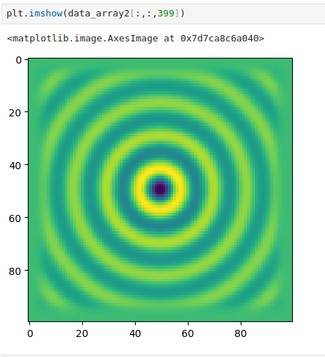
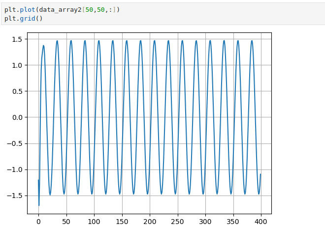
  signal[i] = data_array2[50,50,i]
  auxi1[i] = math.cos(2.0*math.pi*f*time[i])
  auxi2[i] = math.sin(2.0*math.pi*f*time[i])
  auxi3=auxi3+signal[i]*auxi1[i]
  auxi4=auxi4+signal[i]*auxi2[i]
 auxi5 = math.sqrt(auxi3*auxi3+auxi4*auxi4)
 VFT[iff]=auxi5

los archivos h5

Esta es una leccion que aprendimos gracias a chatgpt. Dice que primero ha que instalar “pip install h5py numpy”

import h5py
import numpy as np

# Abre el archivo HDF5 en modo lectura
with h5py.File('eps-000000.00.h5', 'r') as f:
    # Muestra las claves principales del archivo
    print(f"Claves principales del archivo: {list(f.keys())}")

Claves principales del archivo: ['eps']

with h5py.File('eps-000000.00.h5', 'r') as f:
 dataset = f['eps']
 data_array = np.array(dataset)

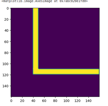
con eso ya se leen los archgivos, por ejemplo, podemos graficar

import matplotlib.pyplot as plt
plt.imshow(data_array)

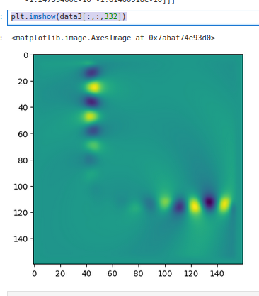
El campo electromagetico tambien lo podemos visualizar si hacemos

# Abre el archivo HDF5 en modo lectura
with h5py.File('ez.h5', 'r') as f:
    # Muestra las claves principales del archivo
    print(f"Claves principales del archivo: {list(f.keys())}")

plt.imshow(data3[:,:,332])

# Abre el archivo HDF5 en modo lectura
with h5py.File('ez.h5', 'r') as f:


 aux1 = f['ez']

# Convierte el dataset a un arreglo de numpy
 aux2 = np.array(aux1)

plt.imshow(data3[:,:,332])

plt.plot(data3[40,40,:])

plt.imshow(data3[40,:,:].transpose())

plt.imshow(data3[:,40,:].transpose())

h5topng -t 0:332 -R -Zc dkbluered -a yarg -A eps-000000.00.h5 ez.h5
convert ez.t*.png ez.gif

A 90 bend

Este es el manual, del manual…, vamos a analizar lo que viene en https://meep.readthedocs.io/en/master/Python_Tutorials/Basics/

# From the Meep tutorial: plotting permittivity and fields of a bent waveguide
import meep as mp

cell = mp.Vector3(16, 16, 0)
geometry = [
    mp.Block(
        mp.Vector3(12, 1, mp.inf),
        center=mp.Vector3(-2.5, -3.5),
        material=mp.Medium(epsilon=12),
    ),
    mp.Block(
        mp.Vector3(1, 12, mp.inf),
        center=mp.Vector3(3.5, 2),
        material=mp.Medium(epsilon=12),
    ),
]
pml_layers = [mp.PML(1.0)]
resolution = 10

sources = [
    mp.Source(
        mp.ContinuousSource(wavelength=2 * (11**0.5), width=20),
        component=mp.Ez,
        center=mp.Vector3(-7, -3.5),
        size=mp.Vector3(0, 1),
    )
]

sim = mp.Simulation(
    cell_size=cell,
    boundary_layers=pml_layers,
    geometry=geometry,
    sources=sources,
    resolution=resolution,
)

sim.run(
    mp.at_beginning(mp.output_epsilon),
    mp.to_appended("ez", mp.at_every(0.6, mp.output_efield_z)),
    until=200,
)

en este ejemplo modificamos la fuente

# From the Meep tutorial: plotting permittivity and fields of a bent waveguide
import meep as mp

cell = mp.Vector3(16, 16, 0)
geometry = [
    mp.Block(
        mp.Vector3(12, 1, mp.inf),
        center=mp.Vector3(-2.5, -3.5),
        material=mp.Medium(epsilon=12),
    ),
    mp.Block(
        mp.Vector3(1, 12, mp.inf),
        center=mp.Vector3(3.5, 2),
        material=mp.Medium(epsilon=12),
    ),
]
pml_layers = [mp.PML(1.0)]
resolution = 10

fcen = 0.15  # pulse center frequency
df = 0.1     # pulse width (in frequency)
sources = [mp.Source(mp.GaussianSource(fcen,fwidth=df),
        component=mp.Ez,
        center=mp.Vector3(-7, -3.5),
        size=mp.Vector3(0, 1),
    )
]

sim = mp.Simulation(
    cell_size=cell,
    boundary_layers=pml_layers,
    geometry=geometry,
    sources=sources,
    resolution=resolution,
)

sim.run(
    mp.at_beginning(mp.output_epsilon),
    mp.to_appended("ez", mp.at_every(0.6, mp.output_efield_z)),
    until=200,
)

se crearon archivos h5, esa fue el output, podemos checar cuales son los archivos con la instrcccion

ls *h5

la cual es valida para cuando esta en el notebook jupyter o cuando estas en el promt en linux, los archivos son dos h5, en el proximo post vamos a ver como se pueden leer en python

eps-000000.00.h5  ez.h5

Autor: new.jmanza@gmail.com

Protegido: Guia recta, caso estacionario, FT

Protegido: Guia recta, pocos pasos

Protegido: Investigacion con meep

doblez3 y la FT como funcion de H