Categoría: Uncategorized

import numpy as np
from scipy.io.wavfile import write
import math
import matplotlib.pyplot as plt
from scipy.signal import stft
from scipy.fft import fft, fftfreq

## PARAMETROS DE LA SENIAL
amplitud = 32767  # Amplitud máxima (para 16-bit PCM)
fs       = 44100  # Frecuencia de muestreo en Hz (común para audio de alta calidad)
ts       = 1/fs
## PARAMETROS DE LA SENIAL

f0       = 330
t0       = 1/f0
ti       = 0.0
tf       = 30*t0
Nt       = int((tf-ti)*fs)
t        = np.zeros(Nt+1)
st       = np.zeros(Nt+1)
fsignal       = np.zeros(Nt+1)
fsignal_i     = 0.5*f0
fsignal_f     = 1.5*f0
dsignal       = (fsignal_f-fsignal_i)/Nt




for it in range(Nt+1):
 t[it]  = ti+it*ts
 fsignal[it] = fsignal_i+it*dsignal
 st[it] = math.sin(2.0*math.pi*fsignal[it]*t[it])

# archivo wav
senal = amplitud*st
senal_int16 = np.int16(senal)
write("senal_sinusoidal.wav", fs, senal_int16)
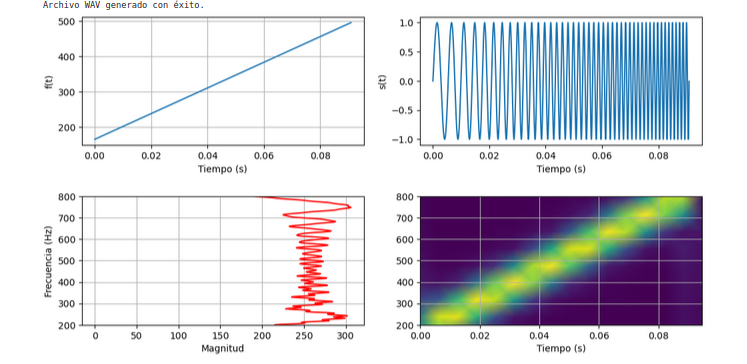
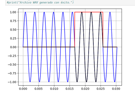
print("Archivo WAV generado con éxito.")



# Zero-padding: Agregar ceros para aumentar la resolución
n_padded = 20096  # Número de puntos para la DFT (aumenta la resolución)
signal_padded = np.pad(st, (0, n_padded - len(st)), 'constant')
# Calcular la DFT
fft_values = fft(signal_padded)
fft_freqs = fftfreq(len(fft_values), 1/fs)

frequencies, times, Zxx = stft(st, fs=fs, nperseg=556)



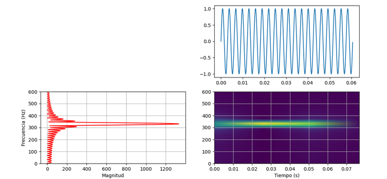
plt.figure(figsize=(12, 6))

plt.subplot(2,2,1)
plt.plot(t,fsignal)
plt.xlabel('Tiempo (s)')
plt.ylabel('f(t)')
plt.grid()

plt.subplot(2, 2, 2)

plt.plot(t,st)
plt.xlabel('Tiempo (s)')
plt.ylabel('s(t)')

#plt.xlabel('Tiempo (s)')

plt.subplot(2, 2, 3)
plt.plot( np.abs(fft_values)[:len(fft_values)//2], fft_freqs[:len(fft_values)//2],'r')
#plt.title("Transformada Discreta de Fourier (DFT)")
plt.ylabel("Frecuencia (Hz)")
plt.xlabel("Magnitud")
plt.ylim([200,800])
plt.grid()

plt.subplot(2,2,4)
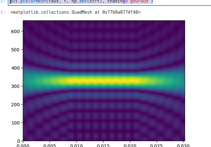
plt.pcolormesh(times, frequencies, np.abs(Zxx), shading='gouraud')
#plt.colorbar(label='Magnitud')
#plt.title('STFT de la Señal Sinusoidal de 330 Hz')
#plt.ylabel('Frecuencia (Hz)')
plt.xlabel('Tiempo (s)')
plt.ylim(200, 800)  # Limitar el rango de frecuencias
plt.grid()
plt.pcolormesh(times, frequencies, np.abs(Zxx), shading='gouraud')


plt.subplots_adjust(hspace=0.4)  

plt.show()

import numpy as np
from scipy.io.wavfile import write
import math
import matplotlib.pyplot as plt

## PARAMETROS DE LA SENIAL
amplitud = 32767  # Amplitud máxima (para 16-bit PCM)
fs       = 44100  # Frecuencia de muestreo en Hz (común para audio de alta calidad)
ts       = 1/fs
## PARAMETROS DE LA SENIAL

f0       = 330
t0       = 1/f0
ti       = 0.0
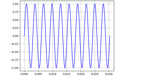
tf       = 10*t0
Nt       = int((tf-ti)*fs)
t        = np.zeros(Nt+1)
st       = np.zeros(Nt+1)

fsignal       = np.zeros(Nt+1)
fsignal_i     = 0.5*f0
fsignal_f     = 1.5*f0
dsignal       = (fsignal_f-fsignal_i)/Nt



for it in range(Nt+1):
 t[it]  = ti+it*ts
 fsignal[it] = fsignal_i+it*dsignal
 st[it] = math.sin(2.0*math.pi*fsignal[it]*t[it])


plt.plot(t,st,'b')

plt.grid()
plt.show()

senal = amplitud*st
senal_int16 = np.int16(senal)
write("senal_sinusoidal.wav", fs, senal_int16)
print("Archivo WAV generado con éxito.")

import numpy as np
from scipy.io.wavfile import write
import math
import matplotlib.pyplot as plt

## PARAMETROS DE LA SENIAL
amplitud = 32767  # Amplitud máxima (para 16-bit PCM)
fs       = 44100  # Frecuencia de muestreo en Hz (común para audio de alta calidad)
ts       = 1/fs
## PARAMETROS DE LA SENIAL

f0       = 330
t0       = 1/f0
ti       = 0.0
tf       = 20*t0
Nt       = int((tf-ti)*fs)
t        = np.zeros(Nt+1)
st       = np.zeros(Nt+1)



for it in range(Nt+1):
 t[it]  = ti+it*ts
 st[it] = math.sin(2.0*math.pi*f0*t[it])


plt.plot(t,st,'b')

plt.grid()
plt.show()

senal = amplitud*st
senal_int16 = np.int16(senal)
write("senal_sinusoidal.wav", fs, senal_int16)
print("Archivo WAV generado con éxito.")

import numpy as np
from scipy.io.wavfile import write
import math
import matplotlib.pyplot as plt
from scipy.signal import stft
from scipy.fft import fft, fftfreq

## PARAMETROS DE LA SENIAL
amplitud = 32767  # Amplitud máxima (para 16-bit PCM)
fs       = 44100  # Frecuencia de muestreo en Hz (común para audio de alta calidad)
ts       = 1/fs
## PARAMETROS DE LA SENIAL

f0       = 330
t0       = 1/f0
ti       = 0.0
tf       = 20*t0
Nt       = int((tf-ti)*fs)
t        = np.zeros(Nt+1)
st       = np.zeros(Nt+1)



for it in range(Nt+1):
 t[it]  = ti+it*ts
 st[it] = math.sin(2.0*math.pi*f0*t[it])

# Zero-padding: Agregar ceros para aumentar la resolución
n_padded = 20096  # Número de puntos para la DFT (aumenta la resolución)
signal_padded = np.pad(st, (0, n_padded - len(st)), 'constant')
# Calcular la DFT
fft_values = fft(signal_padded)
fft_freqs = fftfreq(len(fft_values), 1/fs)

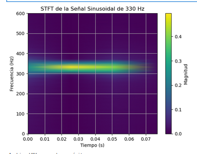
frequencies, times, Zxx = stft(st, fs=fs, nperseg=2256)

plt.pcolormesh(times, frequencies, np.abs(Zxx), shading='gouraud')
plt.colorbar(label='Magnitud')
plt.title('STFT de la Señal Sinusoidal de 330 Hz')
plt.ylabel('Frecuencia (Hz)')
plt.xlabel('Tiempo (s)')
plt.ylim(0, 600)  # Limitar el rango de frecuencias
plt.grid()


plt.show()

senal = amplitud*st
senal_int16 = np.int16(senal)
write("senal_sinusoidal.wav", fs, senal_int16)
print("Archivo WAV generado con éxito.")

plt.plot(fft_freqs[:len(fft_values)//2], np.abs(fft_values)[:len(fft_values)//2], 'r')
plt.title("Transformada Discreta de Fourier (DFT)")
plt.xlabel("Frecuencia (Hz)")
plt.ylabel("Magnitud")
plt.xlim([0,600])
plt.grid()

plt.figure(figsize=(12, 6))

plt.subplot(2, 2, 2)

plt.plot(t,st)

#plt.xlabel('Tiempo (s)')

plt.subplot(2, 2, 3)
plt.plot( np.abs(fft_values)[:len(fft_values)//2], fft_freqs[:len(fft_values)//2],'r')
#plt.title("Transformada Discreta de Fourier (DFT)")
plt.ylabel("Frecuencia (Hz)")
plt.xlabel("Magnitud")
plt.ylim([0,600])
plt.grid()

plt.subplot(2,2,4)
plt.pcolormesh(times, frequencies, np.abs(Zxx), shading='gouraud')
#plt.colorbar(label='Magnitud')
#plt.title('STFT de la Señal Sinusoidal de 330 Hz')
#plt.ylabel('Frecuencia (Hz)')
plt.xlabel('Tiempo (s)')
plt.ylim(0, 600)  # Limitar el rango de frecuencias
plt.grid()
plt.pcolormesh(times, frequencies, np.abs(Zxx), shading='gouraud')

import numpy as np
from scipy.io.wavfile import write
import math
import matplotlib.pyplot as plt


## PARAMETROS DE LA SENIAL
amplitud = 32767  # Amplitud máxima (para 16-bit PCM)
fs       = 44100  # Frecuencia de muestreo en Hz (común para audio de alta calidad)
ts       = 1/fs
## PARAMETROS DE LA SENIAL

f0       = 330
t0       = 1/f0
ti       = 0.0
tf       = 10*t0
Nt       = int((tf-ti)*fs)
t        = np.zeros(Nt+1)
st       = np.zeros(Nt+1)



for it in range(Nt+1):
 t[it]  = ti+it*ts
 st[it] = math.sin(2.0*math.pi*f0*t[it])



plt.plot(t,st,'b')

plt.grid()
plt.show()

senal = amplitud*st
senal_int16 = np.int16(senal)
write("senal_sinusoidal.wav", fs, senal_int16)
print("Archivo WAV generado con éxito.")

import numpy as np
from scipy.io.wavfile import write
import math
import matplotlib.pyplot as plt
from scipy.fft import fft, fftfreq


## PARAMETROS DE LA SENIAL
amplitud = 32767  # Amplitud máxima (para 16-bit PCM)
fs       = 44100  # Frecuencia de muestreo en Hz (común para audio de alta calidad)
ts       = 1/fs
## PARAMETROS DE LA SENIAL

f0       = 330
t0       = 1/f0
ti       = 0.0
tf       = 10*t0
Nt       = int((tf-ti)*fs)
t        = np.zeros(Nt+1)
st       = np.zeros(Nt+1)



for it in range(Nt+1):
 t[it]  = ti+it*ts
 st[it] = math.sin(2.0*math.pi*f0*t[it])

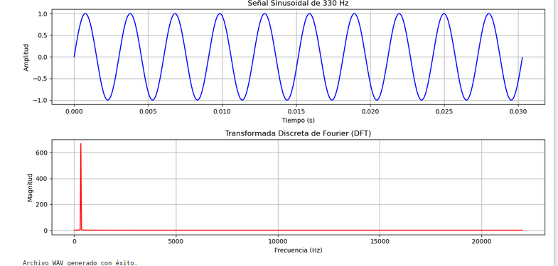
fft_values = fft(st)
fft_freqs = fftfreq(len(fft_values), 1/fs)

# Graficar la señal original
plt.figure(figsize=(12, 6))

plt.subplot(2, 1, 1)
plt.plot(t, st, 'b')
plt.title("Señal Sinusoidal de 330 Hz")
plt.xlabel("Tiempo (s)")
plt.ylabel("Amplitud")
plt.grid()

# Graficar la magnitud de la DFT
plt.subplot(2, 1, 2)
plt.plot(fft_freqs[:len(fft_values)//2], np.abs(fft_values)[:len(fft_values)//2], 'r')
plt.title("Transformada Discreta de Fourier (DFT)")
plt.xlabel("Frecuencia (Hz)")
plt.ylabel("Magnitud")
plt.grid()

plt.tight_layout()
plt.show()

senal = amplitud*st
senal_int16 = np.int16(senal)
write("senal_sinusoidal.wav", fs, senal_int16)
print("Archivo WAV generado con éxito.")

import numpy as np
from scipy.io.wavfile import write
import math
import matplotlib.pyplot as plt
from scipy.fft import fft, fftfreq


## PARAMETROS DE LA SENIAL
amplitud = 32767  # Amplitud máxima (para 16-bit PCM)
fs       = 44100  # Frecuencia de muestreo en Hz (común para audio de alta calidad)
ts       = 1/fs
## PARAMETROS DE LA SENIAL

f0       = 330
t0       = 1/f0
ti       = 0.0
tf       = 10*t0
Nt       = int((tf-ti)*fs)
t        = np.zeros(Nt+1)
st       = np.zeros(Nt+1)



for it in range(Nt+1):
 t[it]  = ti+it*ts
 st[it] = math.sin(2.0*math.pi*f0*t[it])


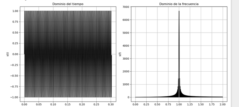
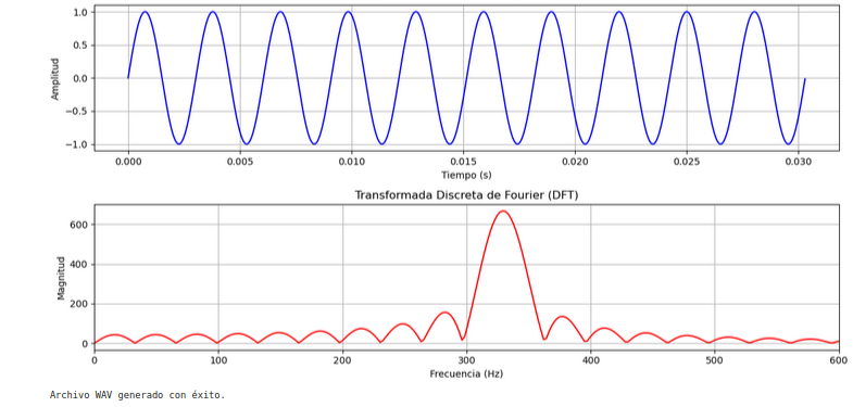
# Zero-padding: Agregar ceros para aumentar la resolución
n_padded = 20096  # Número de puntos para la DFT (aumenta la resolución)
signal_padded = np.pad(st, (0, n_padded - len(st)), 'constant')

# Calcular la DFT
fft_values = fft(signal_padded)
fft_freqs = fftfreq(len(fft_values), 1/fs)



# Graficar la señal original
plt.figure(figsize=(12, 6))

plt.subplot(2, 1, 1)
plt.plot(t, st, 'b')
plt.title("Señal Sinusoidal de 330 Hz")
plt.xlabel("Tiempo (s)")
plt.ylabel("Amplitud")
plt.grid()

# Graficar la magnitud de la DFT
plt.subplot(2, 1, 2)
plt.plot(fft_freqs[:len(fft_values)//2], np.abs(fft_values)[:len(fft_values)//2], 'r')
plt.title("Transformada Discreta de Fourier (DFT)")
plt.xlabel("Frecuencia (Hz)")
plt.ylabel("Magnitud")
plt.xlim([0,600])
plt.grid()

plt.tight_layout()
plt.show()

senal = amplitud*st
senal_int16 = np.int16(senal)
write("senal_sinusoidal.wav", fs, senal_int16)
print("Archivo WAV generado con éxito.")

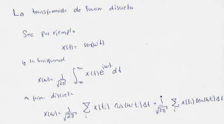
Consideremos el analisis

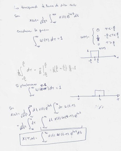
Una buena explicacion del metodo viene en

https://en.wikipedia.org/wiki/Short-time_Fourier_transform

import numpy as np
from scipy.io.wavfile import write
import math
import matplotlib.pyplot as plt

## PARAMETROS DE LA SENIAL
amplitud = 32767  # Amplitud máxima (para 16-bit PCM)
fs       = 44100  # Frecuencia de muestreo en Hz (común para audio de alta calidad)
ts       = 1/fs
## PARAMETROS DE LA SENIAL

f0       = 330
t0       = 1/f0
ti       = 0.0
tf       = 10*t0
Nt       = int((tf-ti)*fs)
t        = np.zeros(Nt+1)
st       = np.zeros(Nt+1)

w        = np.zeros(Nt+1)
tau      = 0.7*tf
B        = 3*t0

for it in range(Nt+1):
 t[it]  = ti+it*ts
 st[it] = math.sin(2.0*math.pi*f0*t[it])
 if t[it] > tau-0.5*B and t[it]<tau+0.5*B:w[it]=1.0


plt.plot(t,st,'b')
plt.plot(t,w,'r')
plt.plot(t,st*w,'k')
plt.grid()
plt.show()

senal = amplitud*st
senal_int16 = np.int16(senal)
write("senal_sinusoidal.wav", fs, senal_int16)
print("Archivo WAV generado con éxito.")

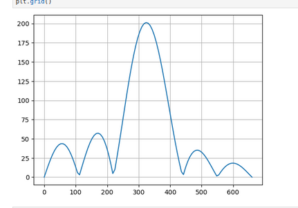
Nf = 100
f  = np.zeros(Nf+1)
sfr = np.zeros(Nf+1)
sfi = np.zeros(Nf+1)
sf  = np.zeros(Nf+1)

fi = 0.0
ff = 2.0*f0
df = (ff-fi)/Nf

for iff in range(Nf+1):
 f[iff] =  fi + iff*df
 for it in range(Nt+1):
  sfr[iff] = sfr[iff]+st[it]*w[it]*math.cos(2.0*math.pi*f[iff]*t[it])
  sfi[iff] = sfi[iff]+st[it]*w[it]*math.sin(2.0*math.pi*f[iff]*t[it])
  sf[iff]  = math.sqrt( sfr[iff]**2 + sfi[iff]**2 )

plt.plot(f,sf)
plt.grid()

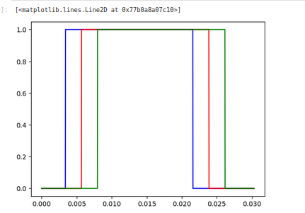
taui = 0.0*tf
tauf = 1.0*tf
Ntau = Nt
dtau = (tauf-taui)/Ntau
tauV = np.zeros(Ntau+1)

w     = np.zeros((Nt+1,Ntau+1))
B     = 6*t0

for itau in range(Ntau+1):
 tauV[itau] = taui+itau*dtau
 for it in range(Nt+1):
  if t[it] > tauV[itau]-0.5*B and t[it]<tauV[itau]+0.5*B:w[it,itau]=1.0

plt.plot(t,w[:,550],'b')
plt.plot(t,w[:,651],'r')
plt.plot(t,w[:,752],'g')

stftr = np.zeros((Nf+1,Ntau+1))
stfti = np.zeros((Nf+1,Ntau+1))
stft  = np.zeros((Nf+1,Ntau+1))

fi = 0.0
ff = 2.0*f0
df = (ff-fi)/Nf
for itau in range(Ntau+1):
 for iff in range(Nf+1):
  f[iff] =  fi + iff*df
  for it in range(Nt+1):
   stftr[iff,itau] = stftr[iff,itau]+st[it]*w[it,itau]*math.cos(2.0*math.pi*f[iff]*t[it])
   stfti[iff,itau] = stfti[iff,itau]+st[it]*w[it,itau]*math.sin(2.0*math.pi*f[iff]*t[it])
   stft[iff,itau]  = math.sqrt( stftr[iff,itau]**2 + stfti[iff,itau]**2 )

plt.pcolormesh(tauV, f, np.abs(stft), shading='gouraud')

from matplotlib.gridspec import GridSpec

# Crear figura
fig = plt.figure(figsize=(10, 10))
gs = GridSpec(2, 2, height_ratios=[1, 1], width_ratios=[1, 2])  # Ajusta la relación de anchos

# Subpanel superior derecho
ax1 = fig.add_subplot(gs[0, 1])  # 2 filas, 2 columnas, segundo panel
ax1.plot(t, st, 'b')
ax1.set_title("Señal en el Tiempo")
ax1.set_xlabel("Tiempo (s)")
ax1.set_ylabel("Amplitud")

# Subpanel inferior derecho
ax2 = fig.add_subplot(gs[1, 0])  # 2 filas, 2 columnas, tercer panel
ax2.plot( -1*sf,f, 'b')
ax2.set_title("Gráfica de -sw")
ax2.set_xlabel("Valor Negativo")
ax2.set_ylabel("Frecuencia")

# Subpanel inferior izquierdo con imshow
ax3 = fig.add_subplot(gs[1, 1])  # Ocupa toda la columna izquierda
#cax = ax3.imshow(stft, cmap='viridis', interpolation='nearest')
cax = ax3.pcolormesh(tauV, f, np.abs(stft), shading='gouraud')
ax3.set_title("STFT")
ax3.set_xlabel("tiempo")
ax3.set_ylabel("frecuencia")
# fig.colorbar(cax, ax=ax3)  # Agregar barra de color si es necesario

plt.tight_layout()
plt.show()

import numpy as np
import math
import matplotlib.pyplot as plt
from scipy.io.wavfile import write

# -> Parámetros de la señal
fs   = 44100 # frecuencia de muestreo
ts   = 1/fs
amplitud = 32767  # Amplitud máxima (para 16-bit PCM)
# -> Parámetros de la señal

f0 = 330     # Frecuencia en Hz (Ejemplo: 440 Hz corresponde a la nota A4)
t0 = 1/f0


ti = 0.0*t0
tf = 10*t0
Nt = int((tf-ti)*fs)
t  = np.zeros(Nt+1)
st = np.zeros(Nt+1)

for it in range(Nt+1):
 t[it] = ti+it*ts
 st[it] = math.sin(2.0*math.pi*f0*t[it])
 
######### -> GENERA WAV
senal_int16 = np.int16(amplitud*st)
# Guardar el archivo WAV
write("aux.wav", fs, senal_int16)
print("Archivo WAV generado con éxito.")
######### -> GENERA WAV


Nf   = 100
fi   = 0.0*f0
ff   = 2.0*f0
df   = (ff-fi)/Nf
f    = np.zeros(Nf+1)
sfr  = np.zeros(Nf+1)
sfi  = np.zeros(Nf+1)
sf   = np.zeros(Nf+1)


for ic in range(Nf+1):
 f[ic] = fi+ic*df
 for it in range(Nt+1):
   sfr[ic] = sfr[ic] + math.cos(2.0*math.pi*f0*t[it])*math.cos(2.0*math.pi*f[ic]*t[it])
   sfi[ic] = sfi[ic] + math.cos(2.0*math.pi*f0*t[it])*math.sin(2.0*math.pi*f[ic]*t[it])

sf = np.sqrt(sfr**2+sfi**2)


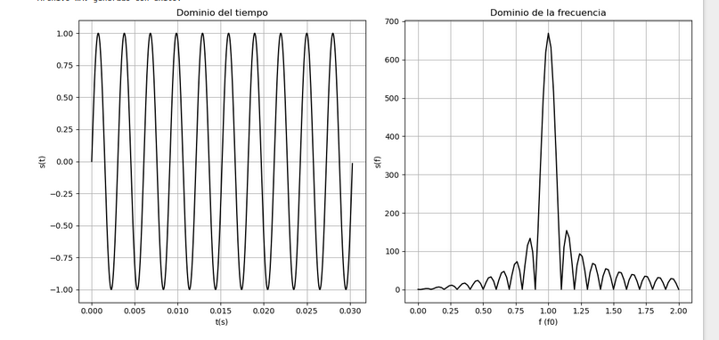
# Graficar la señal original
plt.figure(figsize=(12, 6))

plt.subplot(1, 2, 1)
plt.plot(t , st, 'k')
plt.title('Dominio del tiempo')
plt.xlabel('t(s)')
plt.ylabel('s(t)')
plt.grid()

# Graficar la magnitud de la transformada de Fourier
plt.subplot(1, 2, 2)
plt.plot(f/f0,sf, 'k')
plt.title('Dominio de la frecuencia')
plt.xlabel('f (f0)')
plt.ylabel('s(f)')
plt.grid()
plt.tight_layout()
plt.show()