La transformada discreta de Fourier (home made version)
La transfromada de Fourier (con libreria)
La transformada de Fourier de pulso corto (home made version)
Pagina personal
Esta senial la hacemos con el siguiente programa
import numpy as np
from scipy.io.wavfile import write

# Parámetros de la señal
frecuencia = 2000  # Frecuencia en Hz (Ejemplo: 440 Hz corresponde a la nota A4)
duracion = 5  # Duración en segundos
amplitud = 32767  # Amplitud máxima (para 16-bit PCM)

# Frecuencia de muestreo
fs = 44100  # Frecuencia de muestreo en Hz (común para audio de alta calidad)

# Crear el tiempo de la señal
t = np.linspace(0, duracion, int(fs * duracion), endpoint=False)

# Crear la señal sinusoidal
senal = amplitud * np.sin(2 * np.pi * frecuencia * t)

# Convertir la señal a un formato adecuado para WAV (entero de 16 bits)
senal_int16 = np.int16(senal)

# Guardar el archivo WAV
write("seno_2000.wav", fs, senal_int16)

print("Archivo WAV generado con éxito.")
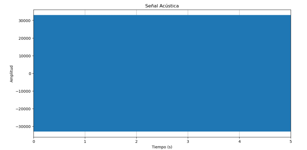
el sonido que sale es este
Para ver esta senial
import numpy as np
import matplotlib.pyplot as plt
from scipy.io import wavfile

# Función para graficar la señal de un archivo WAV
def graficar_senal_wav(archivo_wav):
    # Leer el archivo WAV
    sample_rate, data = wavfile.read(archivo_wav)

    # Comprobar si los datos son estéreo o mono
    if len(data.shape) == 2:
        # Si es estéreo, tomar solo un canal
        data = data[:, 0]

    # Generar el eje de tiempo
    tiempo = np.linspace(0, len(data) / sample_rate, num=len(data))

    # Graficar la señal
    plt.figure(figsize=(12, 6))
    plt.plot(tiempo, data)
    plt.title('Señal Acústica')
    plt.xlabel('Tiempo (s)')
    plt.ylabel('Amplitud')
    plt.grid()
    plt.xlim(0, len(data) / sample_rate)  # Limitar el eje x al tiempo total
    #plt.xlim([2.8,2.85])
    plt.show()

# Especificar el archivo WAV que deseas graficar
from scipy.io import wavfile
from scipy.io import wavfile
archivo_wav = 'seno_2000.wav'  # Cambia esto por el nombre de tu archivo WAV
graficar_senal_wav(archivo_wav)
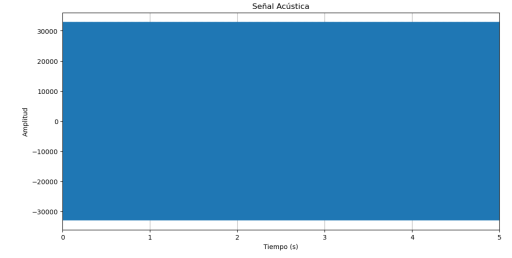
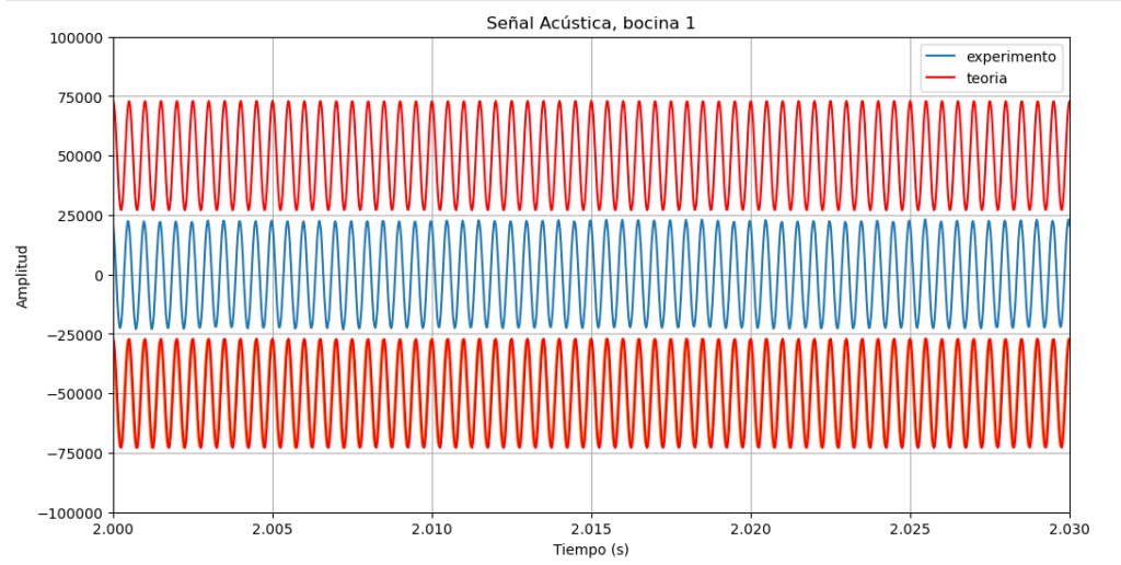
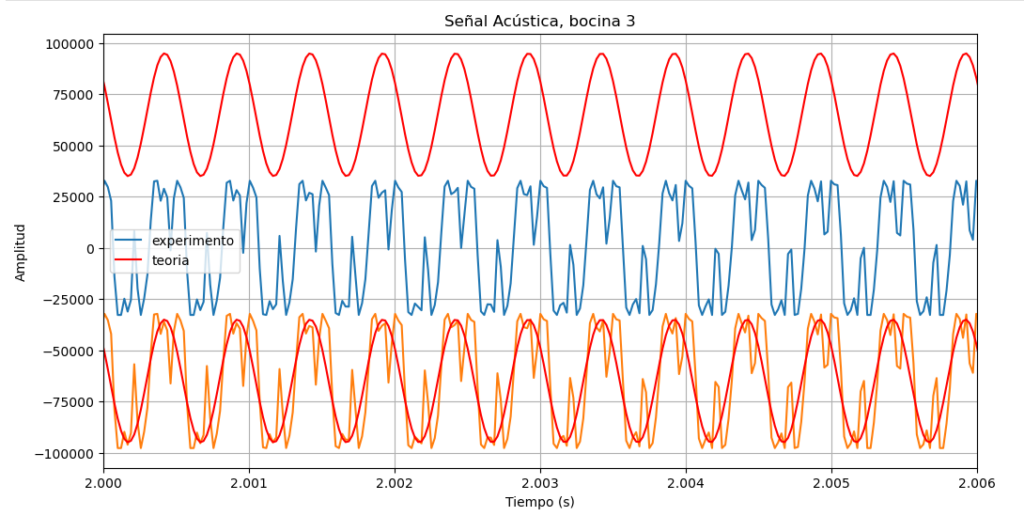
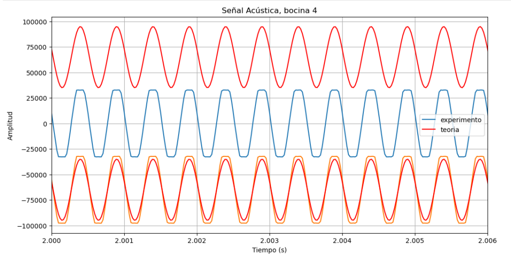
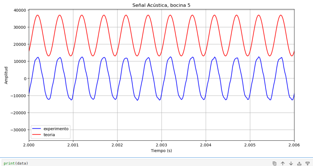
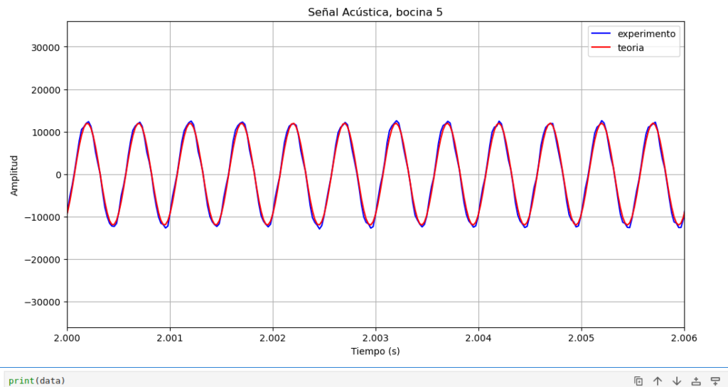
Vamos a analizar como pasa esta onda sinusoidal despues de una bocina y capturandola en un microfono
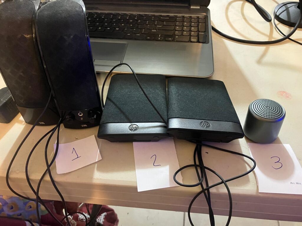
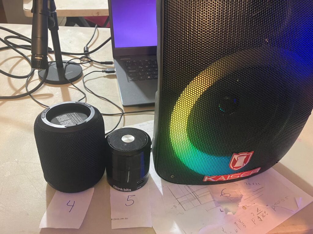
las bocinas registraron los siguientes sonidos, bocina 1
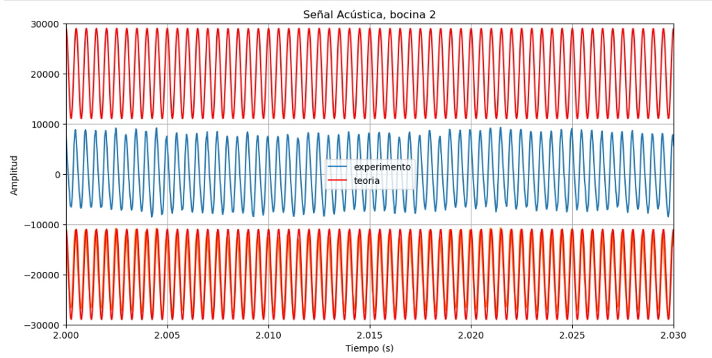
bocina 2
bocina 3
bocina 4
bocina 5
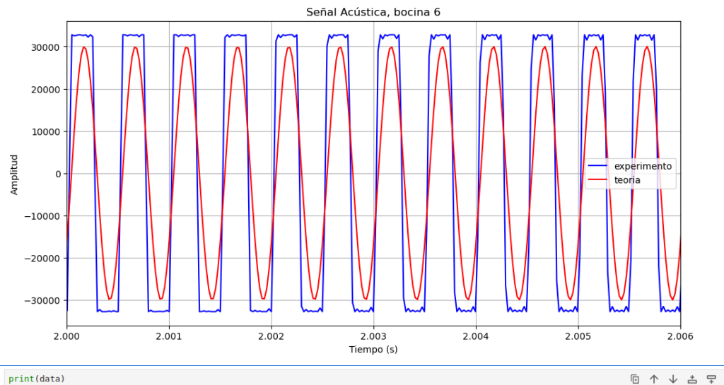
bocina 6
aqui esta la senial de la bocina 1
Podemos generar una senial acustica con l siguiente programa
import numpy as np
from scipy.io.wavfile import write

# Parámetros de la señal
frecuencia = 440  # Frecuencia en Hz (Ejemplo: 440 Hz corresponde a la nota A4)
duracion = 5  # Duración en segundos
amplitud = 32767  # Amplitud máxima (para 16-bit PCM)

# Frecuencia de muestreo
fs = 44100  # Frecuencia de muestreo en Hz (común para audio de alta calidad)

# Crear el tiempo de la señal
t = np.linspace(0, duracion, int(fs * duracion), endpoint=False)

# Crear la señal sinusoidal
senal = amplitud * np.sin(2 * np.pi * frecuencia * t)

# Convertir la señal a un formato adecuado para WAV (entero de 16 bits)
senal_int16 = np.int16(senal)

# Guardar el archivo WAV
write("senal_sinusoidal.wav", fs, senal_int16)

print("Archivo WAV generado con éxito.")
El archivo wav que se genera es el siguiente
Nosotros podemos escuchar ese archivo, ademas, podemos graficarlo mediante el siguiente programa
import numpy as np
import matplotlib.pyplot as plt
from scipy.io import wavfile

# Función para graficar la señal de un archivo WAV
def graficar_senal_wav(archivo_wav):
    # Leer el archivo WAV
    sample_rate, data = wavfile.read(archivo_wav)

    # Comprobar si los datos son estéreo o mono
    if len(data.shape) == 2:
        # Si es estéreo, tomar solo un canal
        data = data[:, 0]

    # Generar el eje de tiempo
    tiempo = np.linspace(0, len(data) / sample_rate, num=len(data))

    # Graficar la señal
    plt.figure(figsize=(12, 6))
    plt.plot(tiempo, data)
    plt.title('Señal Acústica')
    plt.xlabel('Tiempo (s)')
    plt.ylabel('Amplitud')
    plt.grid()
    plt.xlim(0, len(data) / sample_rate)  # Limitar el eje x al tiempo total
    plt.show()

# Especificar el archivo WAV que deseas graficar
archivo_wav = 'senal_sinusoidal1.wav'  # Cambia esto por el nombre de tu archivo WAV
graficar_senal_wav(archivo_wav)
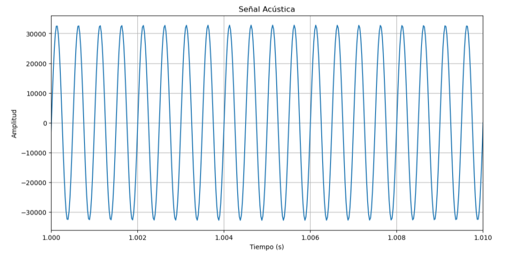
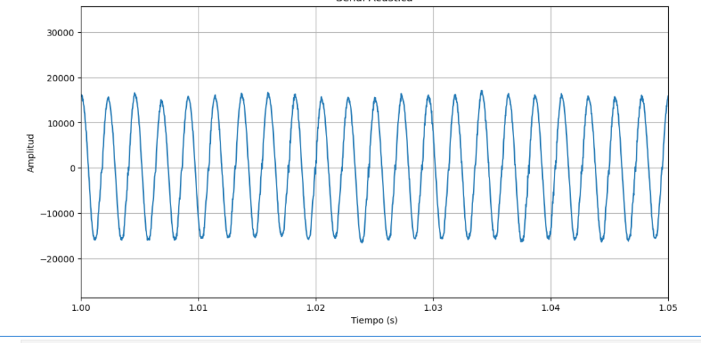
si hacemos un zoom usando plt.xlim([1,1.1]) tenemos
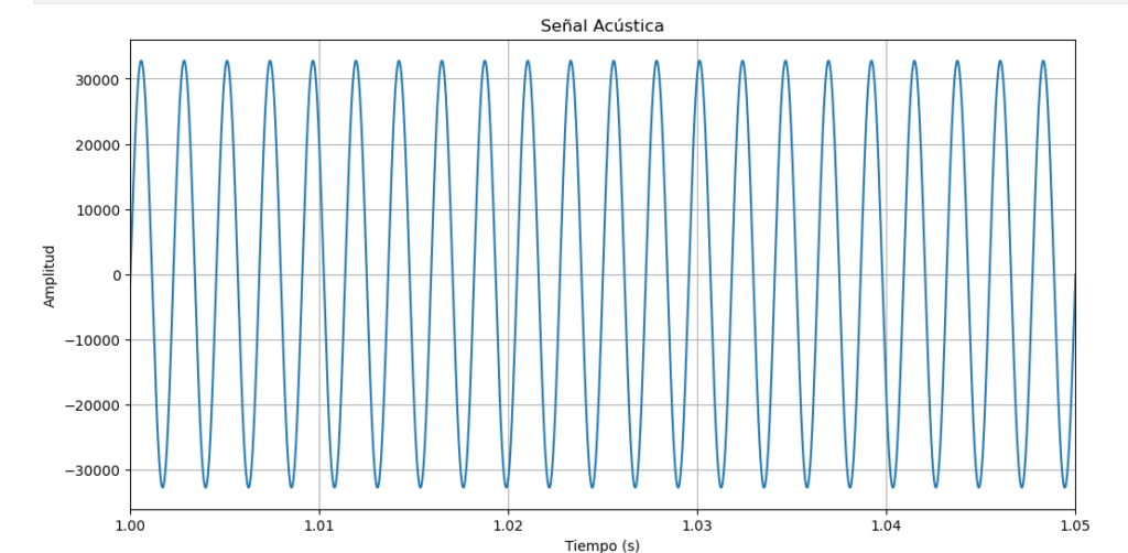
Nos damos cuenta de que esta senial es perfectamente sinusoidal.
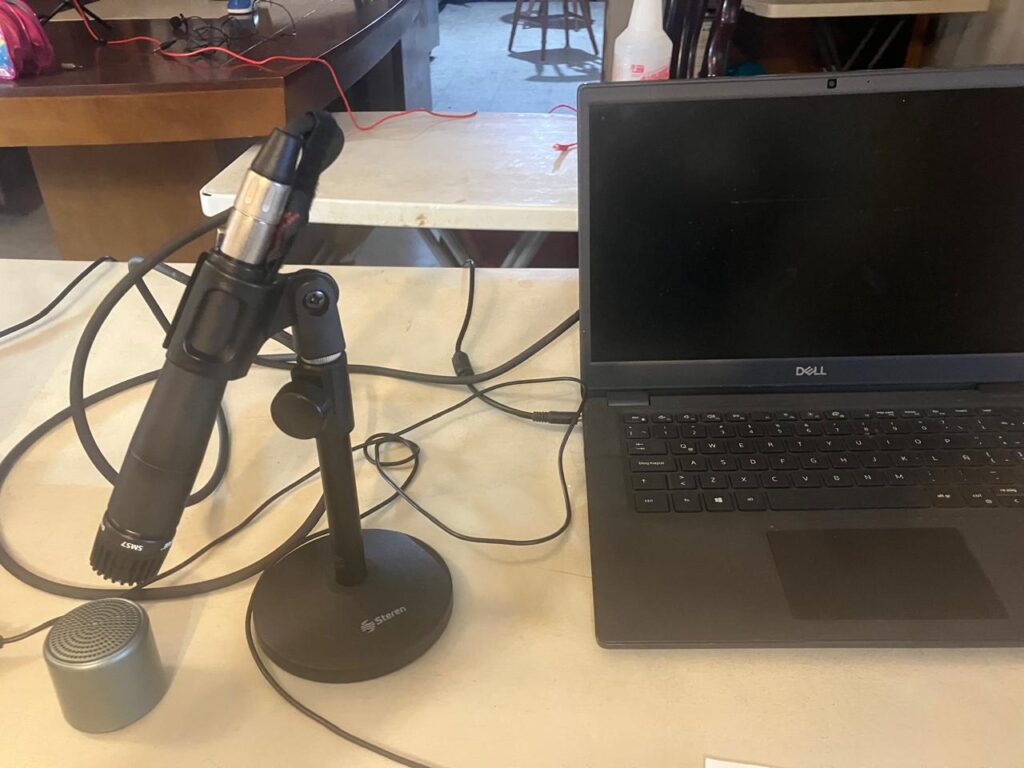
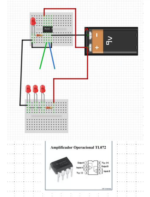
Esta senial genera un archivo wav. Ese archivo wav lo podemos mandar por bluetooth a una bocina. El sonido de la bocina lo podemos grabar con un microfono y generar un nuevo archivo wav.
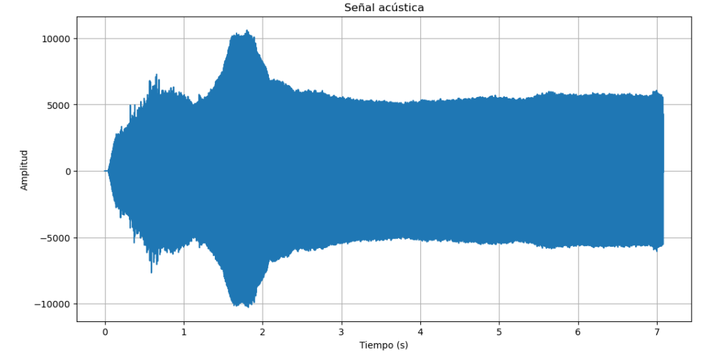
Analizamos este archivo con el mismo programa y obtenemos
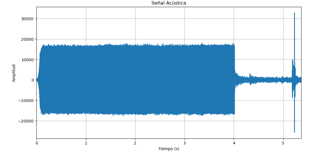
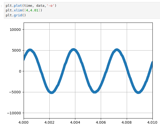
haciendo un zoom tenemos
Esta senial es bastante sinusoidal, es decir, al parecer no pierde mucho calidad.
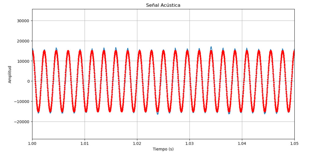
Para convencernos de que la senial es bastante sinusoidal, la comparamos con una senial teorica plt.plot(tiempo,15000np.sin(2.03.1416440tiempo+0.5*3.1416),’.r’)
https://www.dropbox.com/scl/fi/q4xuk6ys1jidw809uh07p/bb.wav?rlkey=96s0aah7o2n7gbcbcu8tdhtry&dl=0
import numpy as np
import matplotlib.pyplot as plt
from scipy.io import wavfile
# Leer el archivo WAV
sample_rate, data = wavfile.read('bb.wav')
# Comprobar si el archivo es estereofónico o monofónico
if len(data.shape) == 2:
    # Si es estereofónico, tomamos solo uno de los canales
    data = data[:, 0]
# Crear un vector de tiempo
time = np.linspace(0, len(data) / sample_rate, num=len(data))
# Graficar la señal
plt.figure(figsize=(12, 6))
plt.plot(time, data)
plt.title('Señal acústica')
plt.xlabel('Tiempo (s)')
plt.ylabel('Amplitud')
plt.grid()
plt.show()
import numpy as np
import scipy.io.wavfile as wav
import matplotlib.pyplot as plt

def calcular_transformada_fourier(archivo_wav):
    # Leer el archivo WAV
    tasa_muestreo, datos = wav.read(archivo_wav)

    # Si el archivo es estéreo (más de un canal), tomamos solo el primer canal
    if len(datos.shape) > 1:
        datos = datos[:, 0]

    # Normalizar los datos para que estén entre -1 y 1
    datos_normalizados = datos / np.max(np.abs(datos), axis=0)

    # Calcular la transformada de Fourier
    transformada = np.fft.fft(datos_normalizados)

    # Obtener las frecuencias correspondientes
    frecuencias = np.fft.fftfreq(len(transformada), 1/tasa_muestreo)

    # Tomamos solo la mitad positiva (frecuencias reales)
    transformada = transformada[:len(transformada)//2]
    frecuencias = frecuencias[:len(frecuencias)//2]

    # Calcular la magnitud (módulo) de la transformada de Fourier
    magnitudes = np.abs(transformada)

    # Graficar el espectro de frecuencias
    plt.figure(figsize=(10, 6))
    plt.plot(frecuencias, magnitudes)
    plt.title('Transformada de Fourier del archivo WAV')
    plt.xlabel('Frecuencia (Hz)')
    plt.ylabel('Magnitud')
    plt.xlim([0,1000])
    plt.grid(True)
    plt.show()

# Nombre del archivo WAV
archivo_wav = 'bb.wav'
calcular_transformada_fourier(archivo_wav)
[\atexpage]
https://www.dropbox.com/scl/fi/6z98nsbu3wuzfffaqjqjf/g.wav?rlkey=ilxj1ygpzawlks88x9tvpnw8k&dl=0
Para leer el arhcivo anterior, usamos
import numpy as np
import matplotlib.pyplot as plt
from scipy.io import wavfile

# Leer el archivo WAV
sample_rate, data = wavfile.read('g.wav')

# Comprobar si el archivo es estereofónico o monofónico
if len(data.shape) == 2:
    # Si es estereofónico, tomamos solo uno de los canales
    data = data[:, 0]

# Crear un vector de tiempo
time = np.linspace(0, len(data) / sample_rate, num=len(data))

# Graficar la señal
plt.figure(figsize=(12, 6))
plt.plot(time, data)
plt.title('Señal acústica')
plt.xlabel('Tiempo (s)')
plt.ylabel('Amplitud')
plt.grid()
plt.show()
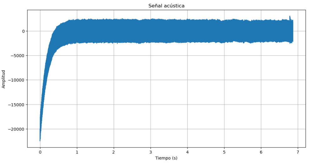
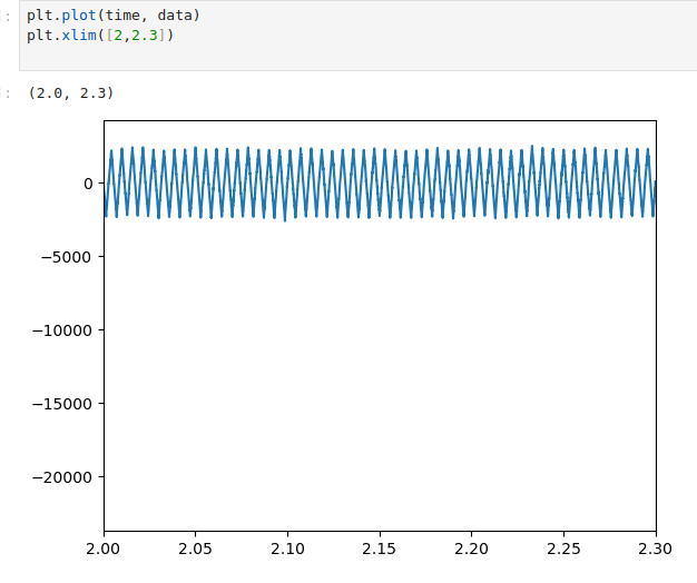
Para obervar que tenemos un seno, hacemos un zoom a la grafica
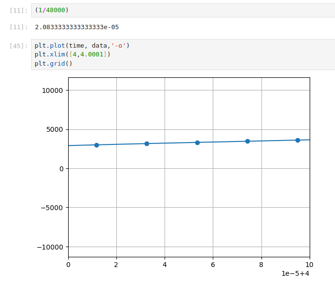
La instruccion sample_rate define la frecuencia a la cual se toman los datos, el periodo con el cual se toman es $\tau_d$ = 1/sample_rate=2.08e-5 seg, en la sigueinte grafica
senial sinusoidal de 5 segundos (440 Hz)
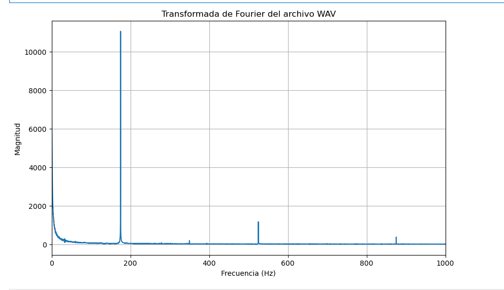
Sacando la transformada de Fourier usando chat gpt