lab_completo capacitor_dielectrico

import numpy as np
import matplotlib.pyplot as plt
import matplotlib.colors as mcolors

# ══════════════════════════════════════════════════════
# PARAMETROS QUE EL ESTUDIANTE PUEDE MODIFICAR
# ══════════════════════════════════════════════════════
d  = 1.0   # separacion entre placas [cm]
V0 = 9.0   # voltaje de la fuente    [V]

# ══════════════════════════════════════════════════════
# MALLA Y POTENCIAL
# ══════════════════════════════════════════════════════
y = np.linspace(0, d, 300)   # eje vertical [cm]
x = np.linspace(0, 1, 10)    # eje horizontal (sin fisica, solo para el mapa)
Y, X = np.meshgrid(y, x)
V = V0 * (1 - Y / d)         # V(y) = V0(1 - y/d)

# ══════════════════════════════════════════════════════
# FIGURA
# ══════════════════════════════════════════════════════
fig, ax = plt.subplots(figsize=(5, 6))

# mapa de color azul -> blanco
cmap = mcolors.LinearSegmentedColormap.from_list('azul_blanco',
                                                  ['white', 'steelblue'])
im = ax.imshow(V.T, origin='upper',
               extent=[0, 1, d, 0],
               cmap=cmap, vmin=0, vmax=V0,
               aspect='auto')

# curvas de nivel (equipotenciales)
niveles = np.linspace(0, V0, 9)[1:-1]   # excluye los extremos (las placas)
cs = ax.contour(X, Y, V, levels=niveles,
                colors='steelblue', linewidths=0.8, linestyles='--', alpha=0.6)
ax.clabel(cs, fmt='%.1f V', fontsize=8, inline=True)

# placas (lineas negras gruesas)
ax.axhline(0, color='black', lw=5, solid_capstyle='round')
ax.axhline(d, color='black', lw=5, solid_capstyle='round')

# flechas E
for xf in [0.25, 0.50, 0.75]:
    ax.annotate("", xy=(xf, d*0.85), xytext=(xf, d*0.15),
                arrowprops=dict(arrowstyle='->', color='navy', lw=1.6))
ax.text(0.82, d/2, r'$\vec{E}$', va='center', fontsize=13, color='navy')

# etiquetas
ax.text(1.03, 0,  f'$V_0 = {V0}$ V', va='center',
        fontsize=10, color='steelblue',
        transform=ax.get_yaxis_transform())
ax.text(1.03, d, '0 V', va='center',
        fontsize=10, color='gray',
        transform=ax.get_yaxis_transform())

# colorbar
cbar = fig.colorbar(im, ax=ax, fraction=0.03, pad=0.12)
cbar.set_label('$V$ (V)', fontsize=10)

ax.set_ylabel('$y$  (cm)', fontsize=11)
ax.set_xticks([])
ax.set_title(rf'$V_0={V0}$ V,  $d={d}$ cm  $\Rightarrow$  '
             rf'$E={V0/d/100:.0f}$ V/m', fontsize=11)

plt.tight_layout()
plt.savefig(f'capacitor_color_d{d}cm.png', dpi=150, bbox_inches='tight')
plt.show()

otro

import numpy as np
import matplotlib.pyplot as plt
import matplotlib.patches as mpatches

# ══════════════════════════════════════════════════════════════════════════════
# PARÁMETRO QUE EL ESTUDIANTE PUEDE MODIFICAR
# ══════════════════════════════════════════════════════════════════════════════
d  = 1.0    # separación entre placas [cm]  <-- cambia este valor
V0 = 9.0    # voltaje de la fuente    [V]

# ══════════════════════════════════════════════════════════════════════════════
# CÁLCULO
# ══════════════════════════════════════════════════════════════════════════════
d_m = d * 1e-2              # convertir a metros
E0  = V0 / d_m              # E = V0/d  [V/m]
y   = np.linspace(0, d, 300)  # eje y en cm
V   = V0 * (1 - y / d)      # V(y) = V0(1 - y/d)

# ══════════════════════════════════════════════════════════════════════════════
# FIGURA
# ══════════════════════════════════════════════════════════════════════════════
fig, (ax1, ax2) = plt.subplots(1, 2, figsize=(11, 5))
fig.suptitle(
    rf"Capacitor de placas paralelas  —  $V_0 = {V0}$ V,  $d = {d}$ cm  "
    rf"$\Rightarrow$  $E = V_0/d = {E0:.1f}$ V/m",
    fontsize=12
)

# ── Panel izquierdo: diagrama del sistema ─────────────────────────────────────
ax1.set_xlim(0, 1)
ax1.set_ylim(-0.25, d + 0.25)
ax1.invert_yaxis()              # y=0 arriba, y=d abajo
ax1.set_ylabel("$y$  (cm)", fontsize=11)
ax1.set_xticks([])
ax1.spines[['top','right','bottom']].set_visible(False)
ax1.spines['left'].set_position(('axes', -0.04))

# Placa + (y=0, línea negra gruesa)
ax1.axhline(0, color='black', lw=5, solid_capstyle='round')
ax1.text(1.04, 0, r'$V_0$', va='center', fontsize=12, color='steelblue',
         transform=ax1.get_yaxis_transform())

# Placa − (y=d, línea negra gruesa)
ax1.axhline(d, color='black', lw=5, solid_capstyle='round')
ax1.text(1.04, d, '$0$', va='center', fontsize=12, color='firebrick',
         transform=ax1.get_yaxis_transform())

# Símbolo tierra debajo de la placa −
tierra_y = d + 0.08
for i, ancho in enumerate([0.18, 0.12, 0.06]):
    ax1.plot([0.5 - ancho, 0.5 + ancho],
             [tierra_y + i*0.05, tierra_y + i*0.05],
             color='firebrick',
             lw=2 - i*0.5)

# Flechas de campo E (de y=0 hacia y=d)
for xf in [0.25, 0.50, 0.75]:
    ax1.annotate(
        "", xy=(xf, d * 0.88), xytext=(xf, d * 0.12),
        arrowprops=dict(arrowstyle='->', color='steelblue', lw=1.8)
    )
ax1.text(0.82, d / 2, r'$\vec{E}$', va='center', ha='left',
         fontsize=13, color='steelblue')

# Cota d (flecha doble en el margen izquierdo)
ax1.annotate(
    "", xy=(0.04, d), xytext=(0.04, 0),
    arrowprops=dict(arrowstyle='<->', color='gray', lw=1.2)
)
ax1.text(0.01, d / 2, '$d$', va='center', ha='center',
         fontsize=11, color='gray')

ax1.set_title("Sistema físico", fontsize=11)

# ── Panel derecho: potencial V(y) ─────────────────────────────────────────────
ax2.plot(y, V, color='steelblue', lw=2.5,
         label=r'$V(y) = V_0\left(1 - y/d\right)$')
ax2.fill_between(y, V, alpha=0.10, color='steelblue')

# líneas de referencia
ax2.axhline(V0, color='steelblue', ls=':', lw=1, alpha=0.6)
ax2.axhline(0,  color='firebrick', ls=':', lw=1, alpha=0.6)

# anotaciones en los extremos
ax2.annotate(f'$V(0) = V_0 = {V0}$ V', xy=(0, V0),
             xytext=(d * 0.12, V0 - 1.2), fontsize=9, color='steelblue',
             arrowprops=dict(arrowstyle='->', color='steelblue', lw=0.8))
ax2.annotate(f'$V(d) = 0$ V', xy=(d, 0),
             xytext=(d * 0.55, 1.2), fontsize=9, color='firebrick',
             arrowprops=dict(arrowstyle='->', color='firebrick', lw=0.8))

ax2.set_xlabel("$y$  (cm)", fontsize=11)
ax2.set_ylabel("$V$  (V)",  fontsize=11)
ax2.set_xlim(0, d)
ax2.set_ylim(-1, V0 + 1)
ax2.legend(fontsize=10)
ax2.grid(alpha=0.25)
ax2.set_title("Potencial $V(y)$", fontsize=11)

plt.tight_layout()
plt.savefig(f"capacitor_d{d}cm.png", dpi=150, bbox_inches='tight')
plt.show()
print(f"  d  = {d} cm  →  E = V0/d = {E0:.1f} V/m")

otro

import numpy as np
import matplotlib.pyplot as plt

# ---
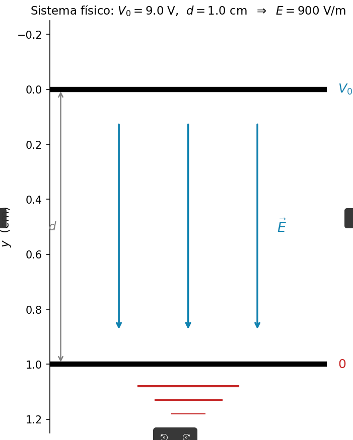
d  = 1.0   # separacion entre placas [cm]  <-- modifica
V0 = 9.0   # voltaje de la fuente    [V]

# ---
E0 = V0 / (d * 1e-2)   # E = V0/d [V/m]

# ---
fig, ax = plt.subplots(figsize=(5, 6))
ax.set_xlim(0, 1)
ax.set_ylim(-0.25, d + 0.25)
ax.invert_yaxis()
ax.set_ylabel("$y$  (cm)", fontsize=11)
ax.set_xticks([])
ax.spines[['top','right','bottom']].set_visible(False)

# placas
ax.axhline(0, color='black', lw=5, solid_capstyle='round')
ax.axhline(d, color='black', lw=5, solid_capstyle='round')

# etiquetas
ax.text(1.04, 0, r'$V_0$', va='center', fontsize=12,
        color='steelblue', transform=ax.get_yaxis_transform())
ax.text(1.04, d, '$0$', va='center', fontsize=12,
        color='firebrick', transform=ax.get_yaxis_transform())

# simbolo tierra
for i, w in enumerate([0.18, 0.12, 0.06]):
    ax.plot([0.5-w, 0.5+w], [d+0.08+i*0.05]*2,
            color='firebrick', lw=2-i*0.5)

# flechas E
for xf in [0.25, 0.50, 0.75]:
    ax.annotate("", xy=(xf, d*0.88), xytext=(xf, d*0.12),
                arrowprops=dict(arrowstyle='->', color='steelblue', lw=1.8))
ax.text(0.82, d/2, r'$\vec{E}$', va='center', fontsize=13, color='steelblue')

# cota d
ax.annotate("", xy=(0.04, d), xytext=(0.04, 0),
            arrowprops=dict(arrowstyle='<->', color='gray', lw=1.2))
ax.text(0.01, d/2, '$d$', va='center', ha='center', fontsize=11, color='gray')

ax.set_title(rf"Sistema físico: $V_0={V0}$ V,  $d={d}$ cm"
             rf"  $\Rightarrow$  $E={E0:.0f}$ V/m", fontsize=11)
plt.tight_layout()
plt.savefig("s1_dibujo_vacio.png", dpi=150, bbox_inches='tight')
plt.show()
print(f"E = V0/d = {E0:.1f} V/m")

otro

import numpy as np
import matplotlib.pyplot as plt
import matplotlib.colors as mcolors

# ---
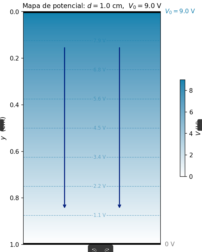
d  = 1.0   # separacion entre placas [cm]  <-- modifica
V0 = 9.0   # voltaje de la fuente    [V]

# ---
y = np.linspace(0, d, 300)
V = V0 * (1 - y / d)
x = np.linspace(0, 1, 10)
Y, X = np.meshgrid(y, x)
V2D  = V0 * (1 - Y / d)

cmap = mcolors.LinearSegmentedColormap.from_list(
    'azul_blanco', ['white', 'steelblue'])

fig, ax = plt.subplots(figsize=(5, 6))
im = ax.imshow(V2D.T, origin='upper', extent=[0,1,d,0],
               cmap=cmap, vmin=0, vmax=V0, aspect='auto')
niveles = np.linspace(0, V0, 9)[1:-1]
cs = ax.contour(X, Y, V2D, levels=niveles,
                colors='steelblue', linewidths=0.8,
                linestyles='--', alpha=0.6)
ax.clabel(cs, fmt='%.1f V', fontsize=8, inline=True)
ax.axhline(0, color='black', lw=5)
ax.axhline(d, color='black', lw=5)
for xf in [0.3, 0.7]:
    ax.annotate("", xy=(xf, d*0.85), xytext=(xf, d*0.15),
                arrowprops=dict(arrowstyle='->', color='navy', lw=1.6))
ax.text(1.03, 0, f'$V_0={V0}$ V', va='center', fontsize=10,
        color='steelblue', transform=ax.get_yaxis_transform())
ax.text(1.03, d, '0 V', va='center', fontsize=10,
        color='gray', transform=ax.get_yaxis_transform())
fig.colorbar(im, ax=ax, fraction=0.03, pad=0.12).set_label('$V$ (V)')
ax.set_ylabel('$y$  (cm)', fontsize=11)
ax.set_xticks([])
ax.set_title(rf"Mapa de potencial: $d={d}$ cm,  $V_0={V0}$ V", fontsize=11)
plt.tight_layout()
plt.savefig("s2_mapa_vacio.png", dpi=150, bbox_inches='tight')
plt.show()

otro

import numpy as np
import matplotlib.pyplot as plt
import matplotlib.colors as mcolors

# ---
d  = 1.0   # separacion entre placas [cm]  <-- modifica
V0 = 9.0   # voltaje de la fuente    [V]

# ---
y = np.linspace(0, d, 300)
V = V0 * (1 - y / d)
x = np.linspace(0, 1, 10)
Y, X = np.meshgrid(y, x)
V2D  = V0 * (1 - Y / d)

cmap = mcolors.LinearSegmentedColormap.from_list(
    'azul_blanco', ['white', 'steelblue'])

fig, ax = plt.subplots(figsize=(5, 6))
im = ax.imshow(V2D.T, origin='upper', extent=[0,1,d,0],
               cmap=cmap, vmin=0, vmax=V0, aspect='auto')
niveles = np.linspace(0, V0, 9)[1:-1]
cs = ax.contour(X, Y, V2D, levels=niveles,
                colors='steelblue', linewidths=0.8,
                linestyles='--', alpha=0.6)
ax.clabel(cs, fmt='%.1f V', fontsize=8, inline=True)
ax.axhline(0, color='black', lw=5)
ax.axhline(d, color='black', lw=5)
for xf in [0.3, 0.7]:
    ax.annotate("", xy=(xf, d*0.85), xytext=(xf, d*0.15),
                arrowprops=dict(arrowstyle='->', color='navy', lw=1.6))
ax.text(1.03, 0, f'$V_0={V0}$ V', va='center', fontsize=10,
        color='steelblue', transform=ax.get_yaxis_transform())
ax.text(1.03, d, '0 V', va='center', fontsize=10,
        color='gray', transform=ax.get_yaxis_transform())
fig.colorbar(im, ax=ax, fraction=0.03, pad=0.12).set_label('$V$ (V)')
ax.set_ylabel('$y$  (cm)', fontsize=11)
ax.set_xticks([])
ax.set_title(rf"Mapa de potencial: $d={d}$ cm,  $V_0={V0}$ V", fontsize=11)
plt.tight_layout()
plt.savefig("s2_mapa_vacio.png", dpi=150, bbox_inches='tight')
plt.show()

otro

import numpy as np
import matplotlib.pyplot as plt
import matplotlib.colors as mcolors

# ---
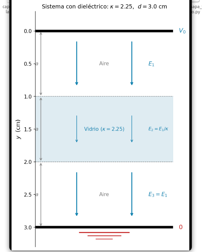
V0    = 9.0    # voltaje [V]
d_cm  = 3.0    # separacion total [cm]
kappa = 2.25   # constante dielectrica

# ---
a   = d_cm / 3.0
a_m = a * 1e-2
E1  = V0 / (a_m * (2 + 1/kappa))
E2  = E1 / kappa
Va  = V0 - E1 * a_m
V2a = Va - E2 * a_m

y  = np.linspace(0, d_cm, 500)
V  = np.where(y <= a,
       V0  - E1 * y * 1e-2,
     np.where(y <= 2*a,
       Va  - E2 * (y-a) * 1e-2,
       V2a - E1 * (y-2*a) * 1e-2))

# malla 2D: Y varia en filas, X en columnas
nx, ny = 10, 400
xv = np.linspace(0, 1, nx)
yv = np.linspace(0, d_cm, ny)
X2D, Y2D = np.meshgrid(xv, yv)          # shape (ny, nx)
V2D = np.where(Y2D <= a,
       V0  - E1 * Y2D * 1e-2,
     np.where(Y2D <= 2*a,
       Va  - E2 * (Y2D-a) * 1e-2,
       V2a - E1 * (Y2D-2*a) * 1e-2))   # shape (ny, nx)

cmap = mcolors.LinearSegmentedColormap.from_list(
    'azul_blanco', ['white', 'steelblue'])

fig, (ax1, ax2) = plt.subplots(1, 2, figsize=(11, 6))
fig.suptitle(rf"$V_0={V0}$ V,  $d={d_cm}$ cm,  $\kappa={kappa}$",
             fontsize=12)

# mapa de color
im = ax1.imshow(V2D, origin='upper', extent=[0,1,d_cm,0],
                cmap=cmap, vmin=0, vmax=V0, aspect='auto')
ax1.axhspan(a, 2*a, color='steelblue', alpha=0.15)
cs = ax1.contour(X2D, Y2D, V2D,
                 levels=np.linspace(0, V0, 10)[1:-1],
                 colors='steelblue', linewidths=0.9,
                 linestyles='--', alpha=0.7)
ax1.clabel(cs, fmt='%.1f V', fontsize=8, inline=True)
for yi in [a, 2*a]:
    ax1.axhline(yi, color='gray', lw=0.8, ls=':')
ax1.axhline(0,    color='black', lw=5)
ax1.axhline(d_cm, color='black', lw=5)
fig.colorbar(im, ax=ax1, fraction=0.03, pad=0.14).set_label('$V$ (V)')
ax1.set_ylabel('$y$  (cm)', fontsize=11)
ax1.set_xticks([])
ax1.set_title('Mapa de potencial', fontsize=11)

# V(y) comparacion
V_ref = V0 * (1 - y / d_cm)
ax2.plot(y, V_ref, color='lightsteelblue', lw=1.5,
         ls='--', label='Sin dielectrico')
ax2.plot(y, V, color='steelblue', lw=2.5,
         label='Con dielectrico')
ax2.axvspan(a, 2*a, color='steelblue', alpha=0.10,
            label=f'Vidrio ($\\kappa={kappa}$)')
for yi, vi in [(a, Va), (2*a, V2a)]:
    ax2.plot(yi, vi, 'o', color='steelblue', ms=6, zorder=5)
    ax2.annotate(f'{vi:.2f} V', xy=(yi, vi),
                 xytext=(yi+0.1, vi+0.5), fontsize=8, color='steelblue')
ax2.axhline(V0, color='steelblue', ls=':', lw=1, alpha=0.5)
ax2.axhline(0,  color='gray',      ls=':', lw=1, alpha=0.5)
ax2.set_xlabel('$y$  (cm)', fontsize=11)
ax2.set_ylabel('$V$  (V)',  fontsize=11)
ax2.set_xlim(0, d_cm)
ax2.set_ylim(-0.5, V0 + 0.5)
ax2.legend(fontsize=9)
ax2.grid(alpha=0.25)
ax2.set_title('Potencial $V(y)$', fontsize=11)

plt.tight_layout()
plt.savefig("s4_mapa_dielectrico.png", dpi=150, bbox_inches='tight')
plt.show()

import numpy as np
import matplotlib.pyplot as plt
import matplotlib.colors as mcolors

# ---
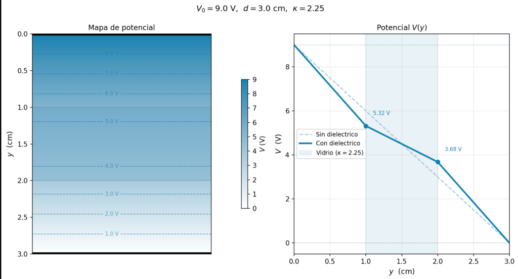
V0    = 9.0    # voltaje [V]
d_cm  = 3.0    # separacion total [cm]
kappa = 2.25   # constante dielectrica

# ---
a   = d_cm / 3.0
a_m = a * 1e-2
E1  = V0 / (a_m * (2 + 1/kappa))
E2  = E1 / kappa
Va  = V0 - E1 * a_m
V2a = Va - E2 * a_m

y  = np.linspace(0, d_cm, 500)
V  = np.where(y <= a,
       V0  - E1 * y * 1e-2,
     np.where(y <= 2*a,
       Va  - E2 * (y-a) * 1e-2,
       V2a - E1 * (y-2*a) * 1e-2))

# malla 2D: Y varia en filas, X en columnas
nx, ny = 10, 400
xv = np.linspace(0, 1, nx)
yv = np.linspace(0, d_cm, ny)
X2D, Y2D = np.meshgrid(xv, yv)          # shape (ny, nx)
V2D = np.where(Y2D <= a,
       V0  - E1 * Y2D * 1e-2,
     np.where(Y2D <= 2*a,
       Va  - E2 * (Y2D-a) * 1e-2,
       V2a - E1 * (Y2D-2*a) * 1e-2))   # shape (ny, nx)

cmap = mcolors.LinearSegmentedColormap.from_list(
    'azul_blanco', ['white', 'steelblue'])

fig, (ax1, ax2) = plt.subplots(1, 2, figsize=(11, 6))
fig.suptitle(rf"$V_0={V0}$ V,  $d={d_cm}$ cm,  $\kappa={kappa}$",
             fontsize=12)

# mapa de color
im = ax1.imshow(V2D, origin='upper', extent=[0,1,d_cm,0],
                cmap=cmap, vmin=0, vmax=V0, aspect='auto')
ax1.axhspan(a, 2*a, color='steelblue', alpha=0.15)
cs = ax1.contour(X2D, Y2D, V2D,
                 levels=np.linspace(0, V0, 10)[1:-1],
                 colors='steelblue', linewidths=0.9,
                 linestyles='--', alpha=0.7)
ax1.clabel(cs, fmt='%.1f V', fontsize=8, inline=True)
for yi in [a, 2*a]:
    ax1.axhline(yi, color='gray', lw=0.8, ls=':')
ax1.axhline(0,    color='black', lw=5)
ax1.axhline(d_cm, color='black', lw=5)
fig.colorbar(im, ax=ax1, fraction=0.03, pad=0.14).set_label('$V$ (V)')
ax1.set_ylabel('$y$  (cm)', fontsize=11)
ax1.set_xticks([])
ax1.set_title('Mapa de potencial', fontsize=11)

# V(y) comparacion
V_ref = V0 * (1 - y / d_cm)
ax2.plot(y, V_ref, color='lightsteelblue', lw=1.5,
         ls='--', label='Sin dielectrico')
ax2.plot(y, V, color='steelblue', lw=2.5,
         label='Con dielectrico')
ax2.axvspan(a, 2*a, color='steelblue', alpha=0.10,
            label=f'Vidrio ($\\kappa={kappa}$)')
for yi, vi in [(a, Va), (2*a, V2a)]:
    ax2.plot(yi, vi, 'o', color='steelblue', ms=6, zorder=5)
    ax2.annotate(f'{vi:.2f} V', xy=(yi, vi),
                 xytext=(yi+0.1, vi+0.5), fontsize=8, color='steelblue')
ax2.axhline(V0, color='steelblue', ls=':', lw=1, alpha=0.5)
ax2.axhline(0,  color='gray',      ls=':', lw=1, alpha=0.5)
ax2.set_xlabel('$y$  (cm)', fontsize=11)
ax2.set_ylabel('$V$  (V)',  fontsize=11)
ax2.set_xlim(0, d_cm)
ax2.set_ylim(-0.5, V0 + 0.5)
ax2.legend(fontsize=9)
ax2.grid(alpha=0.25)
ax2.set_title('Potencial $V(y)$', fontsize=11)

plt.tight_layout()
plt.savefig("s4_mapa_dielectrico.png", dpi=150, bbox_inches='tight')
plt.show()

otro

otro

otro

otro

oto

import numpy as np
import matplotlib.pyplot as plt
import matplotlib.colors as mcolors

—

d = 1.0 # separacion entre placas [cm] <– modifica
V0 = 9.0 # voltaje de la fuente [V]

—

y = np.linspace(0, d, 300)
V = V0 * (1 – y / d)
x = np.linspace(0, 1, 10)
Y, X = np.meshgrid(y, x)
V2D = V0 * (1 – Y / d)

cmap = mcolors.LinearSegmentedColormap.from_list(
‘azul_blanco’, [‘white’, ‘steelblue’])

fig, ax = plt.subplots(figsize=(5, 6))
im = ax.imshow(V2D.T, origin=’upper’, extent=[0,1,d,0],
cmap=cmap, vmin=0, vmax=V0, aspect=’auto’)
niveles = np.linspace(0, V0, 9)[1:-1]
cs = ax.contour(X, Y, V2D, levels=niveles,
colors=’steelblue’, linewidths=0.8,
linestyles=’–‘, alpha=0.6)
ax.clabel(cs, fmt=’%.1f V’, fontsize=8, inline=True)
ax.axhline(0, color=’black’, lw=5)
ax.axhline(d, color=’black’, lw=5)
for xf in [0.3, 0.7]:
ax.annotate(“”, xy=(xf, d0.85), xytext=(xf, d0.15),
arrowprops=dict(arrowstyle=’->’, color=’navy’, lw=1.6))
ax.text(1.03, 0, f’$V_0={V0}$ V’, va=’center’, fontsize=10,
color=’steelblue’, transform=ax.get_yaxis_transform())
ax.text(1.03, d, ‘0 V’, va=’center’, fontsize=10,
color=’gray’, transform=ax.get_yaxis_transform())
fig.colorbar(im, ax=ax, fraction=0.03, pad=0.12).set_label(‘$V$ (V)’)
ax.set_ylabel(‘$y$ (cm)’, fontsize=11)
ax.set_xticks([])
ax.set_title(rf”Mapa de potencial: $d={d}$ cm, $V_0={V0}$ V”, fontsize=11)
plt.tight_layout()
plt.savefig(“s2_mapa_vacio.png”, dpi=150, bbox_inches=’tight’)
plt.show()

import numpy as np
import matplotlib.pyplot as plt

—

d = 1.0 # separacion entre placas [cm] <– modifica
V0 = 9.0 # voltaje de la fuente [V]

—

E0 = V0 / (d * 1e-2) # E = V0/d [V/m]

—

fig, ax = plt.subplots(figsize=(5, 6))
ax.set_xlim(0, 1)
ax.set_ylim(-0.25, d + 0.25)
ax.invert_yaxis()
ax.set_ylabel(“$y$ (cm)”, fontsize=11)
ax.set_xticks([])
ax.spines[[‘top’,’right’,’bottom’]].set_visible(False)

placas

ax.axhline(0, color=’black’, lw=5, solid_capstyle=’round’)
ax.axhline(d, color=’black’, lw=5, solid_capstyle=’round’)

etiquetas

ax.text(1.04, 0, r’$V_0$’, va=’center’, fontsize=12,
color=’steelblue’, transform=ax.get_yaxis_transform())
ax.text(1.04, d, ‘$0$’, va=’center’, fontsize=12,
color=’firebrick’, transform=ax.get_yaxis_transform())

simbolo tierra

for i, w in enumerate([0.18, 0.12, 0.06]):
ax.plot([0.5-w, 0.5+w], [d+0.08+i0.05]2,
color=’firebrick’, lw=2-i*0.5)

flechas E

for xf in [0.25, 0.50, 0.75]:
ax.annotate(“”, xy=(xf, d0.88), xytext=(xf, d0.12),
arrowprops=dict(arrowstyle=’->’, color=’steelblue’, lw=1.8))
ax.text(0.82, d/2, r’$\vec{E}$’, va=’center’, fontsize=13, color=’steelblue’)

cota d

ax.annotate(“”, xy=(0.04, d), xytext=(0.04, 0),
arrowprops=dict(arrowstyle='<->’, color=’gray’, lw=1.2))
ax.text(0.01, d/2, ‘$d$’, va=’center’, ha=’center’, fontsize=11, color=’gray’)

ax.set_title(rf”Sistema físico: $V_0={V0}$ V, $d={d}$ cm”
rf” $\Rightarrow$ $E={E0:.0f}$ V/m”, fontsize=11)
plt.tight_layout()
plt.savefig(“s1_dibujo_vacio.png”, dpi=150, bbox_inches=’tight’)
plt.show()
print(f”E = V0/d = {E0:.1f} V/m”)