import numpy as np
import matplotlib.pyplot as plt
# 1. Configuración de la malla (Aumentamos N para mejor resolución)
N = 500
limit = 3
x = np.linspace(-limit, limit, N)
y = np.linspace(-limit, limit, N)
X, Y = np.meshgrid(x, y)
# 2. Parámetros físicos
q = 1.0
d = 0.6 # Distancia entre cargas
p_vec = np.array([q * d, 0]) # Momento dipolar orientado en X: [px, py]
# 3. Potencial Exacto (Suma de potenciales de dos cargas puntuales)
# Ubicamos la carga positiva en (d/2, 0) y la negativa en (-d/2, 0)
r1 = np.sqrt((X - d/2)**2 + Y**2)
r2 = np.sqrt((X + d/2)**2 + Y**2)
# Usamos un epsilon muy pequeño para evitar la división por cero sin deformar la gráfica
eps = 1e-6
phi_exacto = q * (1.0/np.maximum(r1, eps) - 1.0/np.maximum(r2, eps))
# 4. Potencial Analítico (Aproximación Dipolar para r >> d)
r_mag = np.sqrt(X**2 + Y**2)
# El producto punto p · r se convierte en px*X + py*Y
dot_product = p_vec[0] * X + p_vec[1] * Y
phi_analitico = dot_product / np.maximum(r_mag**3, eps)
# 5. Visualización Profesional
fig, (ax1, ax2) = plt.subplots(1, 2, figsize=(16, 7))
# Configuración de niveles para que ambas gráficas sean comparables
levels = np.linspace(-5, 5, 50)
# Gráfica 1: Potencial Exacto
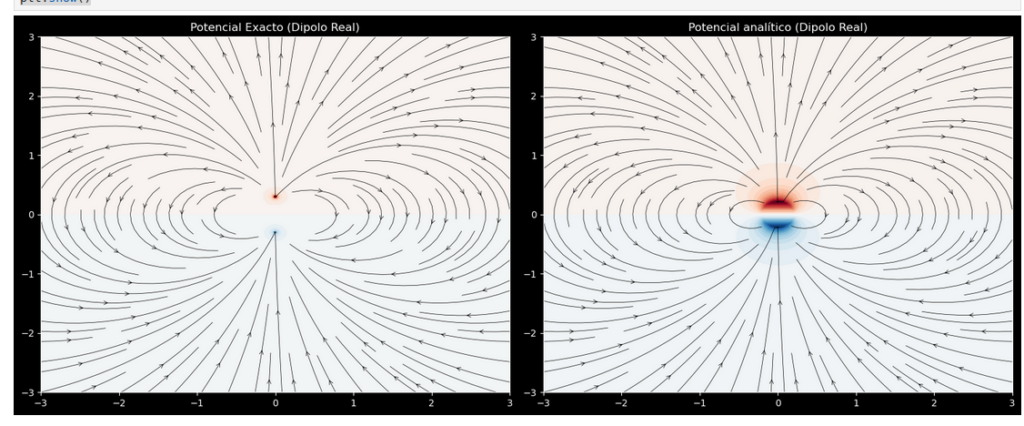
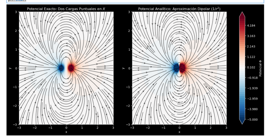
im1 = ax1.contourf(X, Y, phi_exacto, levels=levels, cmap='RdBu_r', extend='both')
# El campo eléctrico es el gradiente negativo del potencial: E = -grad(phi)
# np.gradient devuelve [df/dy, df/dx] para matrices 2D
Ey, Ex = np.gradient(-phi_exacto, y, x)
ax1.streamplot(X, Y, Ex, Ey, color='black', linewidth=0.8, density=1.5, arrowstyle='->')
ax1.set_title("Potencial Exacto: Dos Cargas Puntuales en $X$")
ax1.set_xlabel("x")
ax1.set_ylabel("y")
# Gráfica 2: Potencial Analítico
im2 = ax2.contourf(X, Y, phi_analitico, levels=levels, cmap='RdBu_r', extend='both')
Ey2, Ex2 = np.gradient(-phi_analitico, y, x)
ax2.streamplot(X, Y, Ex2, Ey2, color='black', linewidth=0.8, density=1.5, arrowstyle='->')
ax2.set_title("Potencial Analítico: Aproximación Dipolar ($1/r^2$)")
ax2.set_xlabel("x")
ax2.set_ylabel("y")
fig.colorbar(im1, ax=[ax1, ax2], orientation='vertical', label='Potencial $\Phi$')
plt.show()
import numpy as np
import matplotlib.pyplot as plt
# 1. Configuración de la malla
N = 500
limit = 3
x = np.linspace(-limit, limit, N)
y = np.linspace(-limit, limit, N)
X, Y = np.meshgrid(x, y)
# 2. Parámetros físicos
q = 1.0
d = 0.6 # Distancia entre las cargas
theta = np.radians(30) # Convertir 30 grados a radianes
p_vec = np.array([q * d * np.cos(theta), q * d * np.sin(theta)]) # Momento dipolar
# 3. Potencial Exacto
r1 = np.sqrt((X - d/2 * np.cos(theta))**2 + (Y - d/2 * np.sin(theta))**2)
r2 = np.sqrt((X + d/2 * np.cos(theta))**2 + (Y + d/2 * np.sin(theta))**2)
eps = 1e-6
phi_exacto = q * (1.0/np.maximum(r1, eps) - 1.0/np.maximum(r2, eps))
# 4. Potencial Analítico
r_mag = np.sqrt(X**2 + Y**2)
dot_product = p_vec[0] * X + p_vec[1] * Y
phi_analitico = dot_product / np.maximum(r_mag**3, eps)
# 5. Visualización
fig, (ax1, ax2) = plt.subplots(1, 2, figsize=(16, 7))
levels = np.linspace(-5, 5, 50)
# Gráfica 1: Potencial Exacto
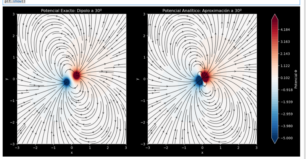
im1 = ax1.contourf(X, Y, phi_exacto, levels=levels, cmap='RdBu_r', extend='both')
Ey, Ex = np.gradient(-phi_exacto, y, x)
ax1.streamplot(X, Y, Ex, Ey, color='black', linewidth=0.8, density=1.5, arrowstyle='->')
ax1.set_title("Potencial Exacto: Dipolo a 30º")
ax1.set_xlabel("x")
ax1.set_ylabel("y")
# Gráfica 2: Potencial Analítico
im2 = ax2.contourf(X, Y, phi_analitico, levels=levels, cmap='RdBu_r', extend='both')
Ey2, Ex2 = np.gradient(-phi_analitico, y, x)
ax2.streamplot(X, Y, Ex2, Ey2, color='black', linewidth=0.8, density=1.5, arrowstyle='->')
ax2.set_title("Potencial Analítico: Aproximación a 30º")
ax2.set_xlabel("x")
ax2.set_ylabel("y")
fig.colorbar(im1, ax=[ax1, ax2], orientation='vertical', label='Potencial $\Phi$')
plt.show()